Shared course · by demo

Statistics for A/B Testing

Design an experiment, work out how long it has to run, and read the result honestly — including the ways a significant result can still be wrong.

lessons
64
to learn
20h 2m
questions
210
written
64/64
Start reading IntermediateEnglish

The path

WrittenNot yet

  1. The logic of hypothesis testing30 min4 questions
  2. One-sided vs two-sided tests15 min3 questions
  3. Fisher vs Neyman-Pearson frameworks20 min3 questions
  4. Null and alternative hypotheses15 min3 questions
  5. Type I and Type II errors15 min3 questions
  6. Test statistics and sampling distributions20 min3 questions
  7. P-value intuition15 min3 questions
  8. Randomization and experimental control25 min4 questions

Lesson 1

The logic of hypothesis testing

You will be able to state a null and alternative hypothesis for an A/B test and describe the two types of error. Covers the concept of a test statistic, the sampling distribution under the null, and the intuition behind the p-value. Prevents treating a non-significant result as proof of no effect.

30 min4 assessments

You've run an A/B test for a week. Variant B shows a 2% higher conversion rate than the control. Is that real improvement, or could it be just random noise? Hypothesis testing gives you a disciplined way to decide — with a known risk of being wrong.

The core idea is simple: assume nothing has changed, then see if your data is too extreme to fit that assumption. The assumption of 'no real difference' is called the null hypothesis (H₀). For an A/B test, H₀ might state: 'the true conversion rate of variant B equals that of variant A' (or the difference is zero). The alternative hypothesis (H₁) is what you're trying to prove: 'the two rates are different' (for a two-sided test) or 'B is better' (one-sided).

You collect data and compute a test statistic — a single number that summarizes the difference between groups, such as the difference in conversion rates. Now the question: if H₀ were true, how likely would you be to see a test statistic as extreme as the one you observed? The answer comes from the sampling distribution under the null: the distribution of the test statistic if the null were true and you repeated the experiment many times. This distribution is derived from probability theory (often the normal distribution via the Central Limit Theorem) or from simulation.

The p-value is the probability, under the null distribution, of getting a test statistic at least as extreme as what you observed. A small p-value (below your chosen significance level α, typically 0.05) means your data is unlikely under H₀ — you reject H₀ in favor of H₁. If the p-value is not small, you fail to reject H₀. Crucially, you never 'accept' H₀; you only conclude that the evidence is insufficient to discard it.

Two types of error can occur. A Type I error (false positive) is rejecting H₀ when it's actually true — you claim a lift that doesn't exist. The significance level α is the probability of a Type I error you're willing to tolerate. A Type II error (false negative) is failing to reject H₀ when H₁ is true — you miss a real effect. The probability of a Type II error is β, and power = 1 − β is the probability of detecting a real effect. These errors trade off: to reduce one, you usually increase the other, unless you increase sample size.

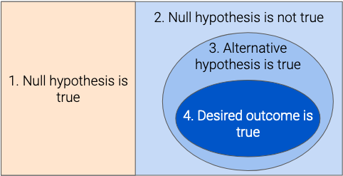
Hypothesis testing decision process and the two types of error. The p-value is compared to the significance level α to decide whether to reject the null hypothesis.

Analogy

Hypothesis testing is like a criminal trial. The null hypothesis is 'the defendant is innocent'. The evidence is the data you collect. The jury's verdict is the decision: 'guilty' (reject H₀) if the evidence is strong enough beyond reasonable doubt, or 'not guilty' (fail to reject H₀) if the evidence is insufficient. The significance level α corresponds to the standard of proof: a stricter court demands stronger evidence to convict, just as a lower α requires a smaller p-value. A Type I error is convicting an innocent person; a Type II error is acquitting a guilty person.

Where the analogy breaks down

In a criminal trial, the consequences of Type I and Type II errors are extremely asymmetric: convicting an innocent person is considered far more harmful than acquitting a guilty one. In hypothesis testing, the researcher chooses α and β deliberately, often balancing them so that both error types are acceptable, and can adjust the trade-off by changing sample size or design. Also, a 'not guilty' verdict does not mean the person is innocent, but the legal system treats it as a final state; in testing, a non-significant result is never proof of H₀ — you simply lack evidence against it.
Go deeper

Watch the short video for a visual, intuitive walkthrough. Then read the textbook chapter for a thorough, step-by-step breakdown of the hypothesis testing process, including the logic of the null distribution and the meaning of the p-value. Note how the video and chapter reinforce the same ideas — the video builds intuition, the chapter formalizes it.

Common misconception

“A p-value of 0.03 means there is only a 3% chance that the null hypothesis is true.”

A small p-value leads to rejecting the null, so it feels like the null is unlikely. The intuition 'if the data is rare under the null, then the null is probably false' is a natural but incorrect reversal of conditional probability.

What is actually true

The p-value is the probability of observing data as extreme as yours (or more) given that H₀ is true — written P(data or more extreme | H₀). It is not the probability that H₀ is true given the data — that would be P(H₀ | data), a quantity that depends on prior beliefs and requires Bayes' theorem. Confusing these two probabilities is the most common error in interpreting statistical results, and it leads directly to overconfidence in findings.

Check yourself

Check your understanding of the logic behind hypothesis testing.

1Multiple choiceChecked instantly

Which statement correctly describes the null hypothesis in an A/B test comparing conversion rates?

  • AThe null hypothesis states that there is a meaningful difference between the variants.
  • BThe null hypothesis states that the observed difference is due to chance and there is no real difference.
  • CThe null hypothesis states that variant B is better than variant A.
  • DThe null hypothesis states that the experiment is designed correctly.
2Short answerMarked by AI

An e-commerce company runs an A/B test to see if a new checkout button increases the purchase rate. They set α = 0.05 and after collecting data they get a p-value of 0.07. (a) State the null and alternative hypotheses for this test (using appropriate notation for proportions). (b) Should they reject the null hypothesis? (c) If they mistakenly reject the null, what type of error would that be? (d) If they fail to reject the null but the new button actually does increase purchases, what type of error have they made?

Graded on Correct formulation of H₀ and H₁ · Correct decision based on p-value vs α · Accurate identification of Type I and II errors

3Short answerMarked by AI

A data scientist runs an A/B test with α = 0.01 and obtains a p-value of 0.003. They claim 'this result is highly statistically significant, so the new feature definitely causes a large improvement.' Evaluate this claim. What can you conclude from the p-value alone? What additional information would you need to judge practical importance?

Graded on Correct interpretation of statistical significance · Identification of missing information · Acknowledgment of limitations and assumptions

4EssayMarked by AI

A product manager runs an A/B test on a new landing page. The p-value is 0.15, so they conclude 'the new page is no better than the old one — we can roll it out to everyone safely.' Write a short essay (200-400 words) explaining why this conclusion is problematic. Specifically: (1) What does 'fail to reject H₀' actually mean? (2) Why can't a non-significant result prove that the null hypothesis is true? (3) What other factors and statistics should be considered before making a business decision?

Graded on Correct interpretation of failing to reject H₀ · Reasons why non-significance does not validate H₀ · Additional factors for business decision

Lesson 2

One-sided vs two-sided tests

You will be able to choose between a one-sided and two-sided alternative and justify the choice. Covers the impact on power and the p-value, and when a one-sided test is appropriate. Prevents using a one-sided test to double significance after seeing the data.

15 min3 assessments

The choice between a one-sided and two-sided test hinges on whether you care about a direction of effect or any difference at all. The table below shows how they differ on the axes that actually matter for planning and interpreting your A/B test.

One-sided (upper tail)

Direction of effect assumed
Tests only if treatment > control
P-value calculation
Area in one tail of the null distribution
Statistical power
Higher for a true effect in the predicted direction; zero for the opposite direction
Ethical constraint
Must be pre-specified before collecting data

Best for When you only care about an increase (e.g., new feature must improve conversion; a decrease is no worse than current)

One-sided (lower tail)

Direction of effect assumed
Tests only if treatment < control
P-value calculation
Area in one tail of the null distribution
Statistical power
Higher for a true effect in the predicted direction; zero for the opposite direction
Ethical constraint
Must be pre-specified before collecting data

Best for When you only care about a decrease (e.g., reducing error rate; an increase is irrelevant or impossible)

Two-sided

Direction of effect assumed
Tests if treatment differs from control (either direction)
P-value calculation
Double the smaller one-sided p-value
Statistical power
Lower than a one-sided test for a given sample size, because it splits α across both tails
Ethical constraint
Default choice; no need to commit to a direction; guards against surprise effects

Best for When you have no strong prior belief about direction, or you need to detect an effect in either direction (e.g., a new pricing page could increase or decrease revenue)

A/B test on checkout button colour

You run an A/B test with 1,000 visitors per variant. The current (control) checkout button has a 5% click-through rate. The new (treatment) button gets 5.5%. You want to know if there is a statistically significant difference.

Two-sided test:

  • Null: p_treatment = p_control
  • Alternative: p_treatment ≠ p_control
  • Using a normal approximation, the z-score is 1.55, giving a two-sided p-value of 0.12.
  • At α = 0.05, you do not reject the null.

One-sided (upper tail) test:

  • Null: p_treatment ≤ p_control
  • Alternative: p_treatment > p_control
  • Same z-score, but the p-value is the area in only the upper tail: 0.06.
  • At α = 0.05, you would reject the null — but only if you had pre-registered that you only care about an increase.

The trap: If you originally planned a two-sided test and then switch to one-sided after seeing the 5.5% > 5%, your effective α becomes 0.10 (because you are choosing the tail that favours you). The correct two-sided p-value is 0.12 — not significant.

Common misconception

“"I should use a one-sided test because it gives more power and a smaller p-value."”

A one-sided test does have higher power for an effect in the predicted direction, and its p-value is half that of the two-sided test for the same observed difference. So it looks like a shortcut to significance.

What is actually true

The power advantage and smaller p-value are only valid if you pre-specified the direction before seeing the data. If you decide the direction after peeking at the results, the true Type I error rate doubles — you are effectively testing at α = 0.10 instead of 0.05. The ethical and statistical requirement is to commit to the test type in your preregistration or analysis plan.

  • A one-sided test detects an effect in only one direction; a two-sided test detects an effect in either direction.
  • The two-sided p-value is always exactly twice the smaller one-sided p-value (for symmetric null distributions).
  • One-sided tests have higher statistical power for an effect in the predicted direction, but zero power for the opposite direction.
  • Switching from a two-sided to a one-sided test after seeing the data inflates the Type I error rate and invalidates the p-value.
  • The choice must be made before collecting data and documented in a preregistration or analysis plan.
  • Two-sided tests are the default in most scientific fields because they are conservative and do not require a directional assumption.
  • YouTube

    One-Tailed vs Two-Tailed Hypothesis Tests | 2-sided vs lower and upper tails

    This short video visualises the difference between one-tailed and two-tailed tests using sampling distributions, making the p-value doubling and power trade-off immediately clear.

    Joshua Emmanuel·3:41·en

    Open
Check yourself

Check your understanding of when and how to choose between one-sided and two-sided tests.

1Multiple choiceChecked instantly

Which of the following is a valid reason to use a one-sided test in an A/B experiment?

  • AThe observed treatment effect was larger than expected.
  • BThe experiment was designed to detect only an increase in the metric.
  • CThe two-sided p-value was 0.09, so switching to one-sided gives significance.
  • DOne-sided tests are always more appropriate than two-sided tests.
2Select all that applyChecked instantly

A colleague reports a one-sided p-value of 0.03 for an A/B test that was originally planned as a two-sided test. Which of the following are true consequences? (Select two.)

  • AThe true Type I error rate for the test is now 6%.
  • BThe result is still valid because the p-value is below 0.05.
  • CThe test is no longer a valid hypothesis test at the 0.05 level.
  • DThe conclusion should be reported with caution because the test was changed post-hoc.
3Short answerMarked by AI

You are designing an A/B test to see if a new checkout flow reduces cart abandonment. The current abandonment rate is 20%. You only care if the new flow reduces abandonment (not if it increases). State the null and alternative hypotheses, and justify whether a one-sided or two-sided test is appropriate.

Graded on Hypotheses are correctly stated and directional · Justification for one-sided test is clear and includes pre-registration

Lesson 3

Fisher vs Neyman-Pearson frameworks

You will be able to distinguish the Fisherian significance test from the Neyman-Pearson hypothesis test and understand why modern practice blends them. Covers the historical debate and the resulting confusion over p-values. Prevents treating a p-value as a long-run error rate.

20 min3 assessments

When you run an A/B test, you probably calculate a p-value and compare it to 0.05. That single step fuses two rival frameworks that were designed for different purposes — and that fusion is the reason p-values are so often misunderstood.

Fisher’s significance test (1925) was built for a single experiment. You state only a null hypothesis (e.g., “the new button is no better”), compute a test statistic, and get a p-value — the probability of seeing data at least this extreme if the null were true. A small p-value is evidence against the null, but there is no alternative hypothesis, no fixed threshold, and no notion of long-run error. You interpret the evidence in context.

Neyman–Pearson hypothesis testing (1933) was built for repeated decision-making. You must state both a null and a specific alternative hypothesis, choose a fixed significance level α (your maximum acceptable Type I error rate), and compute the power (1 − β) for the alternative. You then reject or fail to reject the null. The decision rule guarantees that in the long run you will make a Type I error at most α% of the time — but it says nothing about the evidence in a single experiment.

Modern practice blends them: researchers set α = 0.05 (Neyman–Pearson), report p-values (Fisher), and often treat p < 0.05 as “significant” while ignoring power and the alternative hypothesis. This hybrid is the source of the confusion. A p-value is not the probability that the null is true, and a single significant result does not guarantee a 5% error rate — that guarantee only holds over many repeated tests.

How it got here
  1. 1925

    Fisher publishes *Statistical Methods for Research Workers*

    Introduced the significance test and p-value as a continuous measure of evidence against the null hypothesis, without requiring an alternative hypothesis or a fixed threshold. Solved the problem of quantifying evidence in a single experiment.

  2. 1933

    Neyman and Pearson publish their joint paper on hypothesis testing

    Formalised a decision-theoretic framework with two hypotheses, fixed α and β error rates, and a rejection region. Solved the problem of controlling long-run error rates when making repeated decisions.

  3. 1935

    Fisher and Neyman clash at the Royal Statistical Society

    Fisher argued that Neyman–Pearson testing was irrelevant to scientific inference because it ignored the evidence in a single experiment; Neyman countered that Fisher’s approach lacked a rational basis for action. The debate exposed the fundamental incompatibility of the two frameworks.

  4. 1950s–1960s

    Textbooks blend the two frameworks

    Authors began teaching p-values alongside fixed α thresholds, often without explaining the philosophical differences. Solved the pedagogical problem of having one simple procedure, but created the confusion that persists today.

  5. 2016

    American Statistical Association releases statement on p-values

    Formally warned that p-values are not the probability that the null hypothesis is true, and that statistical significance does not imply practical importance. Highlighted the long-standing misuse caused by the blended framework.

The table below contrasts the two frameworks and the modern hybrid that most researchers actually use.

Fisher’s significance test

Null hypothesis
Required; the only hypothesis
Alternative hypothesis
Not required
Decision rule
No fixed rule; evidence evaluated in context
Error control
None; no long-run guarantee
Interpretation of p-value
Continuous measure of evidence against the null
Role of replication
Each experiment stands alone; evidence accumulates informally

Best for Exploratory research where you want to measure evidence without committing to a decision

Neyman–Pearson hypothesis test

Null hypothesis
Required
Alternative hypothesis
Required; must be specific
Decision rule
Fixed α; reject if p < α, otherwise fail to reject
Error control
Type I error rate controlled at α; Type II error rate controlled by power
Interpretation of p-value
Not used; decision is based solely on whether p < α
Role of replication
Long-run error rates only hold over many repeated tests

Best for Quality control or regulatory settings where a clear accept/reject decision is needed

Modern blended practice

Null hypothesis
Required
Alternative hypothesis
Often vague or omitted
Decision rule
Fixed α (usually 0.05), but p-value is reported as evidence
Error control
α is set, but power is rarely calculated; long-run error rates assumed but not verified
Interpretation of p-value
Treated as both evidence and a decision threshold, causing confusion
Role of replication
Single studies are treated as conclusive, ignoring the need for replication

Best for Convenience; it is the default in most software and journals, despite its flaws

  • Fisher’s significance test uses only a null hypothesis and interprets the p-value as continuous evidence against it, without a fixed decision rule.
  • Neyman–Pearson hypothesis testing requires both a null and a specific alternative, a fixed α, and controls long-run error rates across many experiments.
  • The two frameworks are incompatible in philosophy: one is for measuring evidence, the other for making decisions with known error rates.
  • Modern practice blends them by setting α = 0.05 (Neyman–Pearson) while reporting p-values (Fisher), leading to widespread misinterpretation.
  • A p-value is not the probability that the null hypothesis is true, nor does a single p < 0.05 guarantee a 5% error rate in that experiment.
  • The 2016 ASA statement on p-values explicitly warns against treating p-values as error probabilities or as measures of practical importance.
Go deeper
Check yourself

Check your understanding of the two frameworks and their blend.

1Multiple choiceChecked instantly

Which of the following is a core feature of Fisher's significance test?

  • AIt requires a specific alternative hypothesis.
  • BIt uses a fixed alpha level of 0.05.
  • CIt treats the p-value as evidence strength against the null.
  • DIt controls the long-run Type II error rate.
2Put in orderChecked instantly

Arrange the following historical events in chronological order.

  • AFisher publishes 'Statistical Methods for Research Workers'
  • BNeyman and Pearson publish their joint paper on hypothesis testing
  • CThe ASA releases a statement on p-values
  • DFisher and Neyman debate at the Royal Statistical Society
3Short answerMarked by AI

A colleague runs an A/B test, gets a p-value of 0.04, and says 'There's only a 4% chance the null hypothesis is true.' Explain why this interpretation is incorrect from the Neyman-Pearson perspective, and state what the p-value actually means in that framework.

Graded on Identifies the misinterpretation · States the correct meaning of the p-value in Neyman-Pearson

Lesson 4

Null and alternative hypotheses

Formulating null and alternative hypotheses for A/B tests, including notation and the logic of falsification.

15 min3 assessments
Checklist
0/6

Hypothesis formulation checklist

Keep this open in a second window while you set up your next A/B test. Tick each item before you declare results.

Exercise3 checks
python

Complete the function ab_test_decision so it:

  1. 1.Computes a two-sample t-test (use ttest_ind) on the control and treatment data arrays.
  2. 2.Extracts the p-value from the result.
  3. 3.Returns ('reject', p_value) if p_value < alpha, otherwise ('fail_to_reject', p_value).

Then test it with:

  • Control: 120 conversions out of 1000 visitors
  • Treatment: 150 conversions out of 1000 visitors
  • alpha = 0.05

Your function should return ('reject', 0.0355) (approximately).

Your code must satisfy

  • ab_test_decision(120, 1000, 150, 1000, 0.05)→["reject",0.0355]rejects when difference is large
  • ab_test_decision(120, 1000, 130, 1000, 0.05)→["fail_to_reject",0.4739]fails to reject when difference is small
  • ab_test_decision(120, 1000, 150, 1000, 0.01)→["fail_to_reject",0.0355]respects a stricter alpha
starter code19 lines
from scipy.stats import ttest_ind

def ab_test_decision(control_conversions, control_total, treatment_conversions, treatment_total, alpha=0.05):
    """
    Given conversion counts and totals for control and treatment groups,
    compute the p-value from a two-proportion z-test and return
    ('reject', p_value) or ('fail_to_reject', p_value).
    """
    # Convert counts to arrays of 0s and 1s
    control_data = [1] * control_conversions + [0] * (control_total - control_conversions)
    treatment_data = [1] * treatment_conversions + [0] * (treatment_total - treatment_conversions)
    
    # TODO: compute the p-value using ttest_ind
    p_value = 0.0  # replace this
    
    # TODO: make the decision
    decision = "fail_to_reject"  # replace this
    
    return (decision, round(p_value, 4))

Formulating hypotheses for a checkout button test

Scenario: You are testing whether a green 'Buy Now' button (treatment) converts more visitors than the current blue 'Add to Cart' button (control). You have 5,000 visitors per variant and the current conversion rate is 8%.

  1. 1.Null hypothesis (H₀): The conversion rate is the same for both buttons. H₀: p_control = p_treatment
  1. 2.Alternative hypothesis (H₁): The green button has a different conversion rate. H₁: p_control ≠ p_treatment (two-tailed, because the green button could be worse)
  1. 3.Significance level: α = 0.05
  1. 4.Results after 2 weeks:
  2. 5.Control: 380 conversions out of 5,000 (7.6%)
  3. 6.Treatment: 450 conversions out of 5,000 (9.0%)
  1. 5.Test statistic: observed difference = 9.0% - 7.6% = 1.4 percentage points
  1. 6.p-value: 0.012 (computed via two-proportion z-test)
  1. 7.Decision: Since p = 0.012 < α = 0.05, reject H₀. The data support the alternative that the green button changes conversion rates.

What this means: You have evidence the green button is different. The observed 1.4 percentage point lift is unlikely under the null of no effect. You would now estimate the size of the effect with a confidence interval.

Common misconception

“A p-value of 0.03 means there is a 97% chance the treatment works.”

If p is the probability of seeing the data under the null, and p is small, it feels natural to flip it: 'the null is unlikely, so the alternative is likely.'

What is actually true

The p-value is P(data | H₀), not P(H₀ | data). A p-value of 0.03 means: if H₀ were true, you would see data this extreme only 3% of the time. It does not say there is a 97% chance H₁ is true. To get P(H₀ | data) you need Bayesian methods that incorporate a prior belief about how likely the treatment is to work before the experiment.

The hypothesis testing workflow from question to decision.

Check yourself

Check your understanding of hypothesis formulation and interpretation.

1Put in orderChecked instantly

Arrange these steps in the correct order for conducting a hypothesis test on an A/B experiment.

  • ACompute the p-value
  • BState the null and alternative hypotheses
  • CSet the significance level α
  • DRun the experiment and collect data
  • ECompute the test statistic (observed difference)
  • FCompare p-value to α and make a decision
2Short answerMarked by AI

You run an A/B test comparing two landing page designs. The control has a 5.2% conversion rate, the treatment has a 5.8% conversion rate, and the p-value is 0.08 at α = 0.05. What is your decision and why? Then explain one legitimate reason you might still run the treatment on all traffic despite this result.

Graded on Decision and justification · Legitimate reason to still use the treatment

  • The null hypothesis (H₀) always states no effect or no difference between groups — it is the position you seek evidence against.
  • The alternative hypothesis (H₁) directly contradicts H₀ and can be two-tailed (≠) or one-tailed (> or <) depending on the business question.
  • The significance level α is the false positive rate you accept and must be set before collecting any data.
  • The p-value is P(data | H₀), not P(H₀ | data) — a common misinterpretation that leads to overconfident conclusions.
  • If p < α, reject H₀ in favour of H₁; if p ≥ α, fail to reject H₀ — you never 'accept' the null.
  • A one-tailed test has more power but cannot detect an effect in the opposite direction — choose based on whether the opposite direction matters to your business.

Lesson 5

Type I and Type II errors

Understanding false positives and false negatives, their consequences, and the trade-off between them.

15 min3 assessments

You've written your hypotheses and chosen a test statistic. Now you need to know the two ways your conclusion can be wrong — and they are not symmetrical.

Type I error (false positive) happens when you reject the null hypothesis even though it is true. In an A/B test, this means you conclude the treatment is better when in reality it is no different from the control. The probability of making a Type I error is denoted by α (alpha), and you set it before the test — typically 0.05.

Type II error (false negative) happens when you fail to reject the null hypothesis even though it is false. You miss a real effect. The probability of a Type II error is β (beta). Its complement, 1 − β, is the power of the test — the probability of detecting a real effect of a given size.

These two errors are in tension: reducing α (being more strict about false positives) increases β (you need more evidence, so you're more likely to miss a real effect). The only way to reduce both simultaneously is to increase the sample size.

The two errors differ in what they cost you and how you control them.

Type I error (false positive)

Definition
Rejecting a true null hypothesis
Symbol
α (alpha)
Consequence
You launch a change that doesn't actually work — wasted effort, possible user harm
Control
Set α before the test (e.g., 0.05). Lower α reduces false positives but increases false negatives.
Best for
When false positives are expensive (e.g., deploying a risky feature)

Best for Situations where acting on a false signal is costly

Type II error (false negative)

Definition
Failing to reject a false null hypothesis
Symbol
β (beta)
Consequence
You miss a genuine improvement — lost opportunity, competitor advantage
Control
Increase sample size or effect size. Power = 1 − β is often set to 0.80.
Best for
When false negatives are expensive (e.g., missing a life-saving drug effect)

Best for Situations where missing a real effect is costly

A/B Test for a New Checkout Button

You run an A/B test comparing a new checkout button (treatment) against the current one (control). Historical data shows a 10% conversion rate on the control. You set α = 0.05 and aim for 80% power to detect a 2 percentage point increase (to 12%). You calculate that you need 1,000 users per variant.

Possible outcomes (assuming the null is true — no real effect):

  • With probability 0.95, you correctly fail to reject the null (true negative).
  • With probability 0.05, you incorrectly reject the null (Type I error).

Possible outcomes (assuming the alternative is true — real 2% lift):

  • With probability 0.80, you correctly reject the null (true positive).
  • With probability 0.20, you fail to reject the null (Type II error).

Now suppose the test runs and you observe a p-value of 0.03. You reject the null and conclude the new button is better. But if there is actually no effect, that conclusion is a Type I error. If there is a real effect, it's a correct decision. The risk of Type I error is baked into your α = 0.05; the risk of Type II error (if the true lift is exactly 2%) is 0.20.

Common misconception

“A p-value of 0.03 means there is only a 3% chance that the null hypothesis is true.”

A small p-value makes the null hypothesis seem unlikely, so it's tempting to interpret it as the probability that the null is false.

What is actually true

The p-value is the probability of observing data as extreme as yours, or more extreme, assuming the null hypothesis is true. It is not the probability that the null is true. To get that, you need a Bayesian approach that incorporates prior beliefs. A p-value of 0.03 means that if the null were true, you'd see data this extreme only 3% of the time — it doesn't tell you directly how plausible the null is.

  • Type I error (false positive) = rejecting a true null hypothesis; probability = α.
  • Type II error (false negative) = failing to reject a false null hypothesis; probability = β.
  • Power = 1 − β = probability of detecting a real effect of a given size.
  • α and β trade off: lowering α increases β unless sample size increases.
  • The practical cost of each error depends on the context: false positives waste resources, false negatives miss opportunities.
Check yourself

Check your understanding of Type I and Type II errors.

1Select all that applyChecked instantly

Which of the following are examples of a Type I error? Select all that apply.

  • AConcluding a new feature improves conversion when it actually doesn't.
  • BFailing to detect a real improvement in conversion.
  • CRejecting a true null hypothesis.
  • DAccepting a false null hypothesis.
2Short answerMarked by AI

You run an A/B test with α=0.05 and power=0.80. The test shows a statistically significant increase in revenue (p=0.02). However, the expected lift is only 0.1%, which your business considers negligible. Which error are you more at risk of committing if you launch the change? Explain your reasoning.

Graded on Identifies the correct error · Explains reasoning with reference to effect size and practical significance · Addresses the trade-off between errors

3Multiple choiceChecked instantly

A p-value of 0.03 means:

  • AThere is a 3% chance that the null hypothesis is true.
  • BIf the null hypothesis were true, the probability of observing data as extreme as yours is 3%.
  • CThere is a 97% chance that the alternative hypothesis is true.
  • DThe test has 97% power.

Lesson 6

Test statistics and sampling distributions

How test statistics like difference in proportions are computed and how their sampling distribution under the null enables inference.

20 min3 assessments

You have a null hypothesis — say, "the new landing page converts at the same rate as the old one." To test it, you need a single number that summarises the difference you actually saw in your experiment. That number is the test statistic.

In an A/B test comparing conversion rates, the natural test statistic is the difference in proportions: \( \hat{p}{B} - \hat{p}{A} \). If the null were true, you wouldn't expect this difference to be exactly zero every time — random variation would produce some spread. The sampling distribution under the null models that spread: it's the distribution of the test statistic you would get if you ran the same experiment over and over, assuming the null is true.

For large enough samples, the Central Limit Theorem tells us that the sampling distribution of the difference in proportions is approximately normal, centered at 0 (the null value), with a standard error you can estimate from the data. Once you know the shape of this distribution, you can ask: "How likely is it that I would see a difference as extreme as the one I observed, if the null were true?" That probability is the p-value — and it's the whole point of the test.

The sampling distribution of the difference in proportions under the null. The observed statistic (1.2%) lies in the right tail; the shaded area is the p-value.

Analogy

Imagine a target shooter who claims they can hit the bullseye. The null hypothesis is that they are just aiming at the center but missing randomly. The test statistic is the distance the arrow lands from the bullseye. The sampling distribution under the null is the distribution of distances you'd see if the shooter were just randomly scattering around the center — a bell curve centered at zero. If the arrow lands far out in the tail, you'd say: "That's very unlikely under the null — maybe the shooter is actually aiming elsewhere."

Where the analogy breaks down

The arrow analogy assumes the shooter's errors are symmetric and independent, like a normal distribution. In real A/B tests, the sampling distribution is only approximately normal when sample sizes are large enough (n > 30 per group). If your sample is tiny, the actual distribution may be skewed, and the p-value based on the normal approximation will be misleading.

Common misconception

“The p-value is the probability that the null hypothesis is true.”

A small p-value makes you think the null is unlikely, so it's natural to equate p-value with the probability of the null being false.

What is actually true

The p-value is the probability of observing data as extreme as yours, assuming the null hypothesis is true. It is not the probability that the null is true. To get that, you'd need a prior probability for the null — which is what Bayesian statistics does. A p-value of 0.03 means: if the null were true, you'd see a result this extreme only 3% of the time. It does not mean there is a 97% chance the alternative is correct.

Calculating the p-value for a conversion rate A/B test

Setup: 1000 users saw the control page, 1000 saw the variant. Control conversions: 50 (5%). Variant conversions: 70 (7%). Difference = 0.02.

Step 1: Pooled proportion under null If the null is true, the true conversion rate is the same for both groups. Estimate it by pooling: \( \hat{p} = \frac{50 + 70}{1000 + 1000} = 0.06 \).

Step 2: Standard error of the difference \( SE = \sqrt{\hat{p}(1-\hat{p})\left(\frac{1}{n_A} + \frac{1}{n_B}\right)} = \sqrt{0.06 \times 0.94 \times \left(\frac{1}{1000} + \frac{1}{1000}\right)} \approx 0.0106 \).

Step 3: Z-score \( z = \frac{0.02 - 0}{0.0106} \approx 1.89 \).

Step 4: p-value For a one-tailed test (expecting variant to be higher), the p-value is the area to the right of 1.89 under the standard normal curve. That's about 0.0294. Since 0.0294 < 0.05, we reject the null — the observed difference is unlikely to have occurred by chance alone.

  • The test statistic (e.g., difference in proportions) is a single number that summarises the experiment's outcome.
  • The sampling distribution under the null describes how the test statistic would vary if the null hypothesis were true.
  • For large samples, the sampling distribution of the difference in proportions is approximately normal (CLT).
  • The p-value is the probability of observing a test statistic as extreme as the one computed, assuming the null hypothesis is true.
  • A small p-value (typically < 0.05) suggests the null is unlikely, but it does not measure the probability that the null is true.
Check yourself

Check your understanding of test statistics and sampling distributions.

1Multiple choiceChecked instantly

What does the sampling distribution of a test statistic under the null represent?

  • AThe distribution of the actual data collected in the experiment.
  • BThe distribution of the test statistic if the null hypothesis were true and the experiment were repeated many times.
  • CThe distribution of the p-value across different experiments.
  • DThe distribution of the effect size in the population.
2Short answerMarked by AI

In an A/B test, you observe a difference in conversion rates of 1.5% with a p-value of 0.04. Explain what the p-value of 0.04 means in terms of the sampling distribution under the null. Do not say it is the probability that the null hypothesis is true.

Graded on Correctly identifies what the p-value refers to (probability of data under null) · Uses the numeric value (0.04) in the explanation · Avoids the common misconception

3Short answerMarked by AI

You run an A/B test with 50 users per group. The observed difference in conversion rates is 10%. The p-value from the normal approximation is 0.03. Explain why this p-value might be unreliable, and what you could do to get a more trustworthy result.

Graded on Identifies the sample size as too small and explains why the normal approximation fails · Proposes a concrete remedy · Connects the remedy to the sampling distribution issue

Lesson 7

P-value intuition

Building intuition for the p-value as the probability of observing data as extreme or more under the null, and common misinterpretations.

15 min3 assessments

A p-value is not the probability that the null hypothesis is true. It is the probability of observing a test statistic as extreme as the one you got (or more extreme) if the null hypothesis is true.

Suppose you run an A/B test with a null hypothesis of no difference. After collecting data, you compute a test statistic (e.g., a t-statistic). The p-value tells you: if the null were true and you repeated the experiment many times, what fraction of those repetitions would produce a result at least as surprising as the one you saw?

A small p-value (typically below 0.05) means the observed data would be very unlikely under the null — so you reject the null. A large p-value means the data are consistent with the null, but does not mean the null is true.

How the p-value emerges from the null distribution

Analogy

Imagine a fair coin (null hypothesis: coin is fair). You flip it 20 times and get 18 heads. The p-value is the probability of getting 18 or more heads (or 2 or fewer) if the coin is fair. That's like asking: if the coin is fair, how often would I see a result this extreme? The answer is tiny — so you reject the fair-coin hypothesis.

Where the analogy breaks down

The analogy works for discrete outcomes like coin flips, but in A/B testing the test statistic often comes from a continuous distribution (e.g., t-distribution). In the continuous case, the *exact* probability of any single value is zero, but the p-value uses the entire tail area, so the idea of 'more extreme' still applies. Also, the analogy suggests the p-value is the probability of the observed result alone, when it is actually the probability of the result or more extreme.

  • The p-value is the probability of observing a test statistic as extreme as the one observed, assuming the null hypothesis is true.
  • A small p-value (e.g., < 0.05) suggests the observed data would be unlikely under the null, leading to rejection of the null.
  • A large p-value does not confirm the null hypothesis; it only means the data are not sufficiently inconsistent with it.
  • The p-value depends on the sample size: larger samples can detect smaller effects, making p-values smaller even for tiny differences.
  • The p-value is not the probability that the null hypothesis is true, nor is it the probability that the alternative hypothesis is true.
  • P-values are uniformly distributed under the null hypothesis (if the test is correctly specified), meaning 5% of all true-null experiments will yield p < 0.05.
Common misconception

“The p-value tells me the probability that the null hypothesis is true.”

When you get a very small p-value, you reject the null – so it feels like the p-value measures how likely the null is given the data.

What is actually true

The p-value conditions on the null being true and asks how surprising the data are under that condition. It does not reverse the probability. To get the probability that the null is true given the data, you would need Bayes' theorem and a prior probability, which the classical p-value framework does not provide.

Check yourself

Test your understanding of the p-value.

1Multiple choiceChecked instantly

In an A/B test, you obtain a p-value of 0.03. Which of the following statements is correct?

  • AThere is a 3% chance that the null hypothesis is true.
  • BIf the null hypothesis were true, the probability of observing a test statistic as extreme as (or more extreme than) yours is 3%.
  • CThe probability of making a Type I error is 3%.
  • DThe alternative hypothesis has a 97% chance of being true.

Graded on Selects the correct definition of p-value (option b) · Demonstrates understanding that p-value conditions on the null

2Short answerMarked by AI

A colleague says, 'We ran A/B test, got a p-value of 0.80, so we can be 80% confident that the null hypothesis is true.' Identify the misinterpretation and explain what the p-value of 0.80 actually means in a sentence.

Graded on Identifies the misinterpretation · Provides correct meaning of p=0.80

3Short answerMarked by AI

Consider two A/B tests: Test A has 100 visitors per variant and a p-value of 0.04; Test B has 10,000 visitors per variant and also a p-value of 0.04. Both tests ran on the same product with the same change. Which test likely found a larger practical effect? Explain why the p-value alone is insufficient to judge practical significance.

Graded on Identifies which test has larger practical effect · Explains why p-value alone is insufficient · Suggests what additional metrics to use

Lesson 8

Randomization and experimental control

You will be able to design an A/B test with proper randomization and a control group, and explain why these are essential. Covers simple random assignment, blocking, and the role of a control in isolating the treatment effect. Prevents confounding that invalidates the entire experiment.

25 min4 assessments

The previous lesson, The logic of hypothesis testing, showed you how to state a null and decide whether to reject it. But a hypothesis test is only as trustworthy as the data it runs on. If you let the treatment group see a new feature during a holiday rush while the control group uses the old feature on a slow Tuesday, any lift you measure is just as likely to be the day of week as the treatment. That is confounding: a difference between groups that existed before the treatment was applied.

Randomization breaks that link. By using a chance process—a coin flip, a random number generator—to decide who gets what, you make the two groups probabilistically similar on every measured and unmeasured characteristic. The control group then becomes a mirror of what the treatment group would have looked like without the treatment. This lesson walks you through the steps to design a randomized A/B test with a control group, in the order they must be done.

A Confounded A/B Test

Imagine you want to test a new sign-up flow. The engineering team deploys it to all users who visit during off-peak hours (8 PM–6 AM) because the database is quieter then. The control stays on the old flow during peak hours. After a week you see a 15% improvement in sign-up rate for the new flow.

Is the new flow better? Probably not—the off-peak users may be more engaged or less distracted. The time of day is confounded with the treatment. The correct approach: assign each user randomly, at any time, to either the new flow or the old flow. Now any difference in sign-up rate can only be due to the flow itself, because the groups have the same distribution of visit times, devices, and every other factor.

Random assignment creates two groups that are exchangeable in expectation; any observed difference can be attributed to the treatment.

Steps
0/6

The following steps guide you through designing an A/B test with proper randomization and a control group. Do them in order.

  1. Define the goal and the metric

    Write down the concrete question (e.g., "Does the new checkout button increase purchase completion?") and the primary metric (e.g., "purchase completion rate"). Also decide the minimum effect size you want to detect (e.g., a 2% absolute lift).

    If the metric is vague or you choose it after seeing the data, you introduce researcher degrees of freedom that inflate false positives.

    The metric is a single numeric quantity that can be computed per user (or session), and you have pre-registered it.

  2. Determine the experiment unit and sample size

    The unit is typically the individual user (or session). Ensure units do not interact in a way that contaminates the other group (e.g., social network effects). Use a sample size calculator (or a later lesson) to find how many units you need for adequate power.

    Using sessions when the same user appears multiple times violates independence and under-estimates variance.

    The unit of randomization matches the unit of analysis, and you have a target number of units before the experiment starts.

  3. Randomly assign units to groups

    For each unit, generate a random number (e.g., via random.random() in Python or Math.random() in JavaScript). Assign units with value < 0.5 to the treatment group, the rest to the control group. For small samples, shuffle the list of all units and take the first half as treatment.

    Using a deterministic rule (alternating, or by user ID parity) can be predictable and allows subtle manipulation; always use a true random or cryptographically random generator.

    The two groups have roughly equal size (within expected binomial variation). For a 50/50 split of 1000 users, expect groups of about 500 ±15.

  4. Set up the control group

    The control group receives the current version (or a placebo). No other features should differ between the groups. If blinding is possible (users do not know which version they see), implement it.

    If the control group receives a different user experience (e.g., an extra delay or an ad) that is not a pure placebo, you are comparing two treatments, not a treatment versus no treatment.

    The only thing that differs between the groups is the intervention under test. Both groups should have the same interface, same prompts, and same content aside from the change.

  5. Run the experiment simultaneously

    Start both groups at the same time, and run them for the same duration. Do not stop early based on interim looks without adjusting for multiple testing.

    Running groups at different times (e.g., treatment in January, control in February) reintroduces time-based confounding.

    Both groups have identical start dates, end dates, and any seasonal events (e.g., sales, holidays) affect both.

  6. Check randomization balance

    Compare key pre-treatment covariates (age, previous activity, device type) between groups using a simple summary or a t-test. If any differ significantly at the 5% level, investigate the randomization procedure for errors (a follow-up lesson covers this thoroughly).

    A single significant test is expected by chance when you test many covariates; look for patterns or large imbalances. Do not adjust the randomization after seeing this check—that invalidates the experiment.

    No covariate shows a standardized difference >0.1 or a p-value <0.001 without a plausible explanation. If a known confound is unbalanced, note it for the analysis.

Checklist
0/8

A/B Test Design Field Checklist

Complete all checks before you compute the final p-value. If a check fails, stop and investigate—do not proceed to the hypothesis test.

  • YouTube

    Randomized Controlled Trials (RCTs)

    Watch this 8-minute explanation of how randomized controlled trials are run in practice; it reinforces the steps you just learned and shows the real-world importance of randomization and controls.

    UNICEF Innocenti·8:56·en

    Open
Exercise4 checks
python

Complete the function random_assign so that:

  • Each element of users appears exactly once in either the treatment list or the control list.
  • The treatment list contains about proportion (a float between 0 and 1) of the users; the control list gets the rest.
  • Use random.shuffle on a copy of users to achieve randomness.
  • The function returns a tuple: (treatment_list, control_list).

Your code must satisfy

  • random_assign([1,2,3], 1.0)→[[1,2,3],[]]All in treatment when proportion = 1
  • random_assign([1,2,3], 0.0)→[[],[1,2,3]]All in control when proportion = 0
  • random_assign([], 0.5)→[[],[]]Empty input
  • (lambda x: len(set(x[0]) & set(x[1])))(random_assign([1,2,3,4,5], 0.5))→0No overlapping elements
starter code5 lines
import random

def random_assign(users, proportion=0.5):
    # TODO
    pass
Check yourself

Check your understanding of the material you just covered.

1Put in orderChecked instantly

Order the steps of designing a randomized A/B test from the first action to the last.

  • ADetermine the experiment unit and ensure their assignments are independent.
  • BDefine the key metric and the minimum effect size you care about.
  • CRun the experiment with both groups at the same time and collect data.
  • DRandomly assign each unit to treatment or control using a random process.
  • ECheck that the groups are balanced on pre-treatment covariates.
2Short answerMarked by AI

Explain why a control group is essential in an A/B test even when you have randomization. Then describe two limitations that a control group alone cannot fix, and what additional measures you would take to address them.

Graded on Explains the role of the control group as a counterfactual · Identifies two distinct limitations of the control group alone · Proposes appropriate additional measures

3Multiple choiceChecked instantly

What problem does randomization primarily solve in an A/B test?

  • ASelection bias (volunteer bias)
  • BConfounding by external factors
  • CLow statistical power
  • DMeasurement error

Lesson 9

Blocking and stratification

You will be able to use blocking to reduce variance when a covariate is known to affect the outcome. Covers how to form blocks and analyze a blocked experiment. Prevents ignoring a covariate that could increase power.

15 min4 assessments

When you run an A/B test, random assignment usually balances covariates between groups, but only on average. In a typical test with 10,000 users, chance imbalance on a strong covariate like device type or subscription tier can add enough noise to hide a real effect. Worse, if that covariate interacts with the treatment, you might mistake a baseline difference for a treatment effect.

Blocking solves this by splitting your sample into homogeneous subgroups (blocks) based on the covariate, then randomly assigning treatments within each block. The result: the treatment and control groups are forced to have the same distribution of that covariate, eliminating it as a source of variance.

After the experiment, you analyze across blocks either by a paired test on block-level means or by including the block as a factor in ANOVA. Because the blocked design removes the between-block variance from the error term, the standard error of the treatment effect shrinks — often dramatically.

When should you block? Any covariate you can measure before the experiment that you expect to affect the outcome. Common candidates: existing user segment, device type, geographic region, baseline metric value. The cost is that each block eats one degree of freedom, so blocking on a weak or irrelevant covariate can actually hurt power.

Device type as a blocking factor in a checkout test

You are testing a new checkout button on an e-commerce site. Past data shows conversion rates differ sharply by device:

  • Mobile users: 5% baseline conversion
  • Desktop users: 12% baseline conversion

You have 1000 users: 800 mobile, 200 desktop. Half get the new button (treatment), half the old (control).

Each user independently gets assigned with 50% probability. The actual numbers might turn out:

GroupMobileDesktop
Treatment390 (48.75%)110 (55%)
Control410 (51.25%)90 (45%)

Treatment group has more desktop users (higher baseline). The raw conversion difference = 0.55(pct in T) – 0.45(pct in C) = +10 percentage points from imbalance alone. The treatment effect is buried in this bias.

Divide users by device, then assign half of each block to treatment:

BlockUsersTreatmentControl
Mobile800400400
Desktop200100100

Now the groups are perfectly balanced on device. The observed conversion rates are:

  • Mobile: treatment 6.2%, control 5.1% → lift = +1.1pp
  • Desktop: treatment 13.1%, control 11.9% → lift = +1.2pp

The block-level lifts are nearly identical. A paired analysis on the two blocks gives a much tighter confidence interval than a two-sample test that treats all users as exchangeable.

Variance comparison (simulated):

  • Simple: SE of lift ≈ 2.5pp, not significant (p = 0.09)
  • Blocked: SE of lift ≈ 0.9pp, significant (p = 0.004)

Blocking turned a borderline effect into a clear signal.

Choosing between simple randomization and blocked randomization depends on what you know about your users before the experiment.

Simple randomization

How it controls covariates
Relies on chance to balance; weak control
Variance of treatment effect estimate
Higher (includes between-block variance)
Analysis method
Two-sample t-test, or regression without block factor
Degrees of freedom used
N − 2 (larger)
Implementation overhead
Minimal – just assign randomly across whole sample

Best for When there is no known strong covariate, or the sample is so large that chance imbalance is negligible.

Blocked randomization

How it controls covariates
Forces balance on blocked variable(s)
Variance of treatment effect estimate
Lower (removes between-block variance from error)
Analysis method
Paired t-test on block means, or ANOVA with block factor
Degrees of freedom used
N − b − 1 (where b = number of blocks)
Implementation overhead
Must identify blocks, assign within each; slightly more complex

Best for When a pre‑experiment covariate is strongly correlated with the outcome, especially if the sample per block is moderate.

Common misconception

“If I block on a variable, my experiment will always have higher power and yield significant results.”

Blocking reduces variance, so the standard error of the treatment effect gets smaller. Smaller standard error means larger t-statistic, which often makes a borderline effect significant.

What is actually true

Blocking also reduces the degrees of freedom in the error term (one per block). In small samples or when the block effect is weak, the loss of degrees of freedom can actually increase the critical t-value, making it harder to reach significance. Blocking helps only when the blocked variable truly explains a meaningful fraction of the outcome variance. If you block on an irrelevant variable (like birthday month), you cost yourself power with no benefit.

Go deeper
Check yourself

Check your understanding of when and how to block.

1Select all that applyChecked instantly

Which of the following are valid reasons to use blocking in an A/B test? (Select all that apply.)

  • AYou have strong evidence that the covariate affects the outcome.
  • BYou want to reduce the variance of the treatment effect estimate.
  • CYou have many covariates and want to use them all, even if they are weak.
  • DYou expect the treatment effect to be identical across all subgroups.
2Multiple choiceChecked instantly

When should you consider NOT using a blocking factor even though you have a measurable pre‑experiment covariate?

  • AWhen the covariate is categorical with more than 10 levels.
  • BWhen the covariate is known to be uncorrelated with the outcome.
  • CWhen the total sample size is less than the number of blocks.
  • DWhen the covariate is continuous and cannot be discretized.
3Short answerMarked by AI

You have a sample of 60 users divided into 15 blocks (4 users per block). The within‑block variance is small, but you see that the block means vary widely. If you treat the experiment as completely randomized (ignoring blocks), you fail to reach significance. After using a blocked analysis (paired t‑test on block means), the p‑value drops to 0.01. Explain why the blocked analysis found a signal that the simple test missed, and identify one risk of using so many blocks with only 4 users each.

Graded on Correctly explains variance source isolation · Identifies the risk of small block size · Connects the scenario to the decision of whether to block

Exercise3 checks
python

Implement analyze_blocked_experiment. The arrays treatment and control contain outcome values from paired units (same block, same size per block). blocks is an integer block ID for each pair. Compute the difference (treatment - control) for each pair, then average those differences within each block. Finally, run a one-sample t-test (using scipy.stats.ttest_1samp) on the block-level differences against 0. Return the p-value. Assume every block has the same number of pairs, but do not assume the blocks are numbered consecutively.

Your code must satisfy

  • analyze_blocked_experiment(np.array([10, 12, 11, 21, 22, 20]), np.array([9, 10, 10, 15, 16, 14]), np.array([0, 0, 0, 1, 1, 1]))→"0.001745"synthetic balanced blocks
  • analyze_blocked_experiment(np.array([5, 5, 5, 5]), np.array([5, 5, 5, 5]), np.array([0, 0, 1, 1]))→"1.0"no effect
  • analyze_blocked_experiment(np.array([1, 2, 3]), np.array([0, 1, 2]), np.array([0, 0, 0]))→"0.5"single block (fallback to paired on raw pairs)
starter code11 lines
from scipy import stats
import numpy as np

def analyze_blocked_experiment(treatment, control, blocks):
    """
    Given arrays of treatment outcomes, control outcomes, and a block label for each pair,
    return the p-value from a paired t-test on block-level differences.
    block: array of length len(treatment) containing integer block IDs.
    """
    # TODO: compute mean difference per block, then run a one-sample t-test
    pass

Lesson 10

A/A tests to validate randomization

You will be able to run an A/A test to check that your randomization procedure is not broken. Covers what to look for in the results and how many A/A tests are enough. Prevents launching an A/B test on a platform that secretly biases assignment.

15 min4 assessments

You just finished an A/B test. The p-value is 0.03. The lift looks real. You start drafting the announcement. But what if the result is a mirage — caused by a broken randomization algorithm, not a genuine effect? That's the exact disaster an A/A test prevents.

An A/A test runs two identical groups (both receive the control variant) and checks whether any metric shows a statistically significant difference. If it does, something is wrong with your experiment platform — the randomization, the data pipeline, or the metric calculation. A/A tests are a low-cost sanity check before you spend weeks or months on a real A/B test.

The most common failures they catch:

  • Sample ratio mismatch (SRM): the groups aren't 50/50. A hash collision, cookie churn, or race condition in the assignment service can silently unbalance the split.
  • Covariate imbalance: users differ systematically between groups on age, location, device, or behavior — often from time-based assignment (e.g., more desktop users assigned to A on weekdays, more mobile users to B on weekends).
  • Tracking asymmetry: an instrumentation bug logs events in group A but drops them in group B.
  • Multiple testing inflation: you peeked at 20 metrics and one happened to be significant.

If a single A/A test shows p < 0.05, you investigate — you don't treat it as a discovery. But even passing one test is not enough; a subtle bias may require more data to surface. The gold standard is to run 10–20 A/A tests and expect around 5% to show significance at α = 0.05, consistent with the expected false positive rate.

  • An A/A test compares two groups that both receive the same treatment to validate that the experiment platform produces false positive rates close to the expected alpha.
  • A statistically significant result in an A/A test indicates a systematic bias in assignment, data collection, or metric calculation — not a real effect.
  • Sample ratio mismatch (SRM) is the most common failure detected by A/A tests; a chi-squared test can confirm whether the observed split deviates from the intended 50/50 beyond random chance.
  • Covariate imbalance (e.g., on age, location, device type) can be detected by comparing distributions between groups; a significant Kolmogorov-Smirnov or chi-squared test on a covariate signals a problem.
  • Running at least 5–10 A/A tests increases the sensitivity to rare biases and allows you to check whether the share of significant results matches the expected false positive rate (e.g., 5% at α = 0.05).
  • If an A/A test fails, you must identify and fix the root cause before proceeding to A/B testing — ignoring it risks launching a change based on an artifact.

Decision tree for diagnosing an A/A test failure. Start at the symptom and trace each branch until you find a cause.

Decide

You work at a subscription service. Your team runs a standard A/A test before every major A/B test: 50/50 split, 10,000 users per group, observe conversion rate for 14 days. Today, the A/A test shows p = 0.04 on conversion rate. A colleague says, 'Great, the treatment might actually work — let's deploy it!'

What is the first thing you should check?

Checklist
0/6

A/A Test Diagnostic Checklist

Use this checklist every time you run an A/A test. A single item failure is enough to halt the pipeline until resolved.

Check yourself

Test your ability to diagnose A/A test results and decide when a randomization pipeline is trustworthy.

1Short answerMarked by AI

You run an A/A test with 10,000 users per group and observe a conversion rate difference with p = 0.04. List three distinct checks you would perform to diagnose the issue, and for each explain what result would indicate a problem.

Graded on Identifies relevant checks · Explains what result indicates a problem

2Select all that applyChecked instantly

Which of the following are valid reasons to run an A/A test? (Select all that apply.)

  • ATo verify that the randomization algorithm is assigning users without systematic bias.
  • BTo estimate the required sample size for a future A/B test.
  • CTo detect instrumentation bugs that cause events to be logged differently between groups.
  • DTo measure the effect size of a known treatment.
  • ETo check that the false positive rate of the experiment platform matches the expected alpha (e.g., 5%).

Graded on Correctness of selections · Avoids wrong options

3Put in orderChecked instantly

Arrange the following steps for conducting and diagnosing an A/A test in the correct chronological order.

  • ADefine one primary metric to monitor.
  • BRun the test with a 50/50 split for a predetermined duration.
  • CCheck sample ratio using a chi-squared test.
  • DCheck covariate balance on key characteristics (age, device, location).
  • ECheck tracking symmetry between groups.
  • FIf any check fails, investigate the root cause and fix; otherwise proceed to A/B tests.

Graded on Order of first four steps · Order of final two steps

4Short answerMarked by AI

You perform five independent A/A tests on your platform. None show a significant result at α = 0.05. Does this guarantee your randomization is perfect? Explain in 2–4 sentences.

Graded on Correctly denies guarantee and explains why · References false positive rate or statistical reasoning

Lesson 11

Simple random assignment

The mechanics of randomly assigning subjects to control and treatment groups using random number generators or physical randomization methods.

15 min1 assessment

You've learned why randomization matters in A/B testing. Now you need to actually do it — assign every incoming user to either the control group or the treatment group, with no pattern, no bias, and no way for you or the system to guess which one comes next.

Simple random assignment means each subject has an equal, independent chance of landing in either group. If you flip a fair coin for every user, that's simple random assignment. The problem is that a coin doesn't scale to thousands of users, and a human flipping it will subconsciously cheat.

You'll use a random number generator (RNG) instead. The standard approach: generate a random number between 0 and 1 for each subject, and assign to treatment if that number is below your split threshold (usually 0.5). The key is that the RNG must be cryptographically secure — not random() in most languages without seeding, because that produces predictable sequences. Python's random.SystemRandom() or secrets module works. JavaScript's crypto.getRandomValues() works. Never use Math.random() for anything that matters — it's a PRNG seeded from the current time, and an attacker or even a coincidental system clock pattern can reproduce your assignments.

You also need to log the assignment before the user sees the variant. If you assign on the fly and the user refreshes, they must get the same group — otherwise you've broken the random assignment and introduced a selection bias (users who refresh more often will see both variants, which changes their behavior). The fix: generate the assignment once, store it in the user's session or a database row, and read it back on every subsequent request.

Steps
0/4

You have 10,000 users arriving over a week. You need to assign each to control or treatment with a 50/50 split. Here's how to do it in Python, step by step.

  1. Choose your RNG

    Import secrets (Python 3.6+). This gives you cryptographically secure random bytes. Do not use random.random() — it's a PRNG and predictable.

    Using `random.seed(0)` or `random.random()` in production makes your assignments reproducible by anyone who knows the seed.

    `secrets.randbelow(100)` returns a number between 0 and 99 inclusive, and it's fast.

  2. Generate the assignment threshold

    python5 lines
    from secrets import randbelow
    # Generate an integer from 0 to 999
    threshold = randbelow(1000)
    # Assign to treatment if threshold < 500 (50% chance)
    is_treatment = threshold < 500

    This is equivalent to a coin flip but uses secure randomness.

    Using `randbelow(1000)` and comparing to 500 gives exactly 50/50. If you use `randbelow(2)` and compare to 0, you get exactly 50/50 but with less granularity — fine for simple assignment.

    Run the snippet 10 times in a loop; you should see roughly 5 True and 5 False.

  3. Log the assignment before the user sees the variant

    python9 lines
    def assign_user(user_id):
        # Check if already assigned
        existing = db.get_assignment(user_id)
        if existing is not None:
            return existing
        # New assignment
        is_treatment = secrets.randbelow(1000) < 500
        db.store_assignment(user_id, is_treatment)
        return is_treatment

    The database lookup happens first, so a returning user always gets the same group.

    If you generate the assignment inside the request handler without checking first, a page refresh re-assigns the user. This breaks randomization.

    Call `assign_user("user_1")` twice; both calls return the same value.

  4. Handle the split ratio

    Change the threshold to adjust the split. For a 10% treatment group, use secrets.randbelow(1000) < 100. For 33%, use < 330 (or < 333 for exact 1/3). The denominator must be a power of 10 or a multiple of your split ratio to avoid rounding bias.

    Using `randbelow(3) < 1` for 33% split is exact but only works for fractions with denominator 3. For 33.3%, use `randbelow(1000) < 333`.

    Run 1000 assignments with threshold 100; count of treatment assignments should be near 100.

Checklist
0/7

Simple Random Assignment Checklist

Use this checklist when setting up any A/B test. Tick each item before you start collecting data.

Exercise2 checks
python

Complete the assign_user function. It should:

  1. 1.Check if user_id is already in the assignments dictionary (provided).
  2. 2.If yes, return the existing assignment.
  3. 3.If no, generate a new assignment using secrets.randbelow(1000) where the threshold is int(treatment_probability * 1000).
  4. 4.Store the new assignment in assignments[user_id].
  5. 5.Return the new assignment.

Example: assign_user("alice", 0.5) should return True or False with roughly 50% probability, and calling it again with the same user_id returns the same value.

Your code must satisfy

  • assignments = {}; a = assign_user('test1', 0.5); b = assign_user('test1', 0.5); a == b→truereturns same value on repeat call
  • assignments = {}; results = [assign_user(f'user{i}', 0.1) for i in range(2000)]; sum(results)→200assigns with correct probability
starter code12 lines
from secrets import randbelow

def assign_user(user_id, treatment_probability):
    """
    Assign a user to treatment (True) or control (False).
    treatment_probability is a float between 0 and 1.
    If the user already has an assignment, return it.
    Otherwise, generate a new assignment, store it, and return it.
    """
    # Assume a dictionary `assignments` exists for storage
    # Your code here
    pass
  • Simple random assignment gives each subject an equal, independent chance of being in control or treatment.
  • Use a cryptographically secure RNG (Python's secrets module) — never random.random() for production A/B tests.
  • Log the assignment before the user sees the variant, and check for an existing assignment on every request.
  • The split ratio is set by changing the threshold in randbelow(1000) < threshold; the denominator must cleanly represent the ratio.
  • A fixed seed or predictable PRNG makes the assignment sequence reproducible and thus not random.
  • Re-randomizing on page refresh breaks the experiment; always store and retrieve the assignment per user.
Go deeper

Read the Wikipedia article on random assignment for a broader view of how this fits into experimental design, including alternative methods like block randomization.

Lesson 12

Control groups and treatment effects

Why a control group is essential to isolate the treatment effect from external factors, and how to define and interpret the treatment effect.

15 min3 assessments

You’ve randomized your users and launched the new feature. A week later the treatment group shows 5.2% conversion. Is that the feature’s doing? Without a control group you have no way to know. Maybe a holiday drove all traffic up; maybe a competitor’s outage pushed users your way. The control group – identical in every way except the treatment – gives you the counterfactual: what would have happened if you hadn’t changed anything.

Formally, the treatment effect is the difference between the outcome in the treatment group and the outcome in the control group. For a binary metric like conversion:

code1 line
Treatment effect (absolute) = conversion_rate_treatment - conversion_rate_control

For revenue or session time you might use a relative change:

code1 line
Relative lift = (mean_treatment - mean_control) / mean_control

Randomization ensures the two groups are comparable on average, but the control group is still the only way to subtract out everything that happened to both groups during the experiment. Without it, you’re guessing.

This builds directly on the randomization you already know from the previous node – but randomization alone isn’t enough. The control group is the anchor that makes the measurement meaningful.

The control group isolates the treatment effect by subtracting the baseline outcome.

Analogy

Think of a medical trial for a new headache drug. The treatment group gets the drug; the control group gets a placebo (a sugar pill). Any improvement in the treatment group could be due to the drug, but it could also be due to the placebo effect – people simply feeling better because they’re being treated. The control group captures the placebo effect, so the true drug effect is the difference between the two groups.

In A/B testing, the “placebo” is your current product. The control group experiences the same external events (seasonality, marketing campaigns, competitor moves) as the treatment group. By comparing the two, you strip away those external factors and see only the effect of the change you made.

Where the analogy breaks down

In a medical trial the placebo is chemically inert, so the difference between groups is a clean estimate of the drug’s effect. In A/B testing the “placebo” (current product) is not inert – it has its own history, user expectations, and ongoing changes. Also, treatment effects in A/B testing are often tiny (fractions of a percent) and require very large samples, whereas drug effects are often larger. The analogy breaks when you assume the control group is a neutral baseline; it’s actually a baseline that itself evolves, so you need to run the experiment long enough to average out its normal fluctuations.

Calculating the treatment effect from a real A/B test

Scenario

An e-commerce team runs an A/B test on the checkout page. They randomly assign 10,000 users to the new design (treatment) and 10,000 to the current design (control). After one week:

GroupVisitorsConversionsConversion Rate
Treatment10,0004204.20%
Control10,0003103.10%

Absolute treatment effect

4.20% - 3.10% = 1.10 percentage points

Relative lift

(4.20% - 3.10%) / 3.10% = 1.10% / 3.10% ≈ 0.3548 = 35.5% increase

Interpretation

The new checkout design lifted conversion by 1.10 percentage points, a 35.5% relative improvement over the current baseline. Note: this is the estimated effect – we haven’t yet checked if it’s statistically significant (that comes later).

Common misconception

“If I randomize properly, I don’t need a control group – I can just compare the treatment group’s result to last month’s average.”

Historical data is readily available and seems to provide a baseline. Randomization already ensures the treatment group is representative, so why run a second group?

What is actually true

Historical data is contaminated by time trends, seasonality, marketing campaigns, and other changes that happened between then and now. A contemporary control group, exposed to the same external conditions, isolates the treatment effect from all those confounding factors. Without a concurrent control, you can’t tell whether the change you see is due to the new feature or to something else that happened at the same time.

Check yourself

Check your understanding of control groups and treatment effects.

1Multiple choiceChecked instantly

Which of the following best describes the purpose of a control group in an A/B test?

  • ATo ensure the treatment group receives the new feature.
  • BTo provide a baseline that accounts for external factors, so the treatment effect can be isolated.
  • CTo increase the sample size and improve statistical power.
  • DTo test multiple variations of the feature simultaneously.
2Short answerMarked by AI

An A/B test of a new checkout flow produces the following results:

Treatment group (n=5,000): 120 conversions Control group (n=5,000): 95 conversions

Calculate the absolute and relative treatment effect. Then write one sentence interpreting what the effect means for the business.

Graded on Correct calculation of absolute effect · Correct calculation of relative lift · Interpretation in business terms

3EssayMarked by AI

Explain why a control group is necessary even when randomization is performed. Include a concrete scenario where a confounding variable (such as a seasonal trend or a marketing campaign) could bias the results if only the treatment group were measured and compared to historical data.

Graded on Explains why control group is necessary despite randomization · Provides a concrete scenario with a confounding variable · Links the scenario to the need for a concurrent control group

Lesson 13

Randomization checks

Statistical tests and visual checks to verify that randomization produced comparable groups on observed covariates.

15 min4 assessments
Decide

You've just run an A/B test on a new checkout flow. The primary metric — conversion rate — shows a statistically significant lift (p = 0.03, +2%). But before you ship, your colleague asks: 'Did you check that the groups are balanced on age?' You pull the data: the control group has an average age of 34.2, the variant 36.8. The difference is 2.6 years. What do you do?

You run a t-test on age between groups and get p = 0.01. What does this tell you?

Decision tree for interpreting a covariate imbalance in an A/B test.

Randomization should make groups comparable on all covariates, but chance imbalances happen. A randomization check tests whether observed differences on key covariates are larger than expected by chance. Common tests: two-sample t-test for continuous covariates, chi-square test for categorical. But beware: testing many covariates inflates the chance of false positives. Focus on covariates known to affect the outcome (e.g., previous purchase history for conversion). If a covariate shows a significant difference with a large effect size, investigate the randomization procedure itself — it may have failed. If the effect size is small, it's likely just noise; you can still proceed but consider adjusting for that covariate in the analysis (e.g., ANCOVA).

Checking age balance in an A/B test

You have 500 users per group. Control mean age = 34.2, variant = 36.8, pooled SD = 10. Compute t-statistic: t = (36.8 - 34.2) / (10 sqrt(1/500 + 1/500)) = 2.6 / (10 0.0632) ≈ 2.6 / 0.632 ≈ 4.11. With df ≈ 998, p ≈ 0.00004. The p-value is very small, but the effect size (Cohen's d = 2.6/10 = 0.26) is small to medium. Given that this is one of several covariates, the small effect size suggests it's likely a chance imbalance, not a procedural failure. However, because the p-value is extreme, you should still verify the randomization logs.

Checklist
0/6

Randomization check checklist

Use this checklist every time you analyze an A/B test. Do not skip it even if the primary metric is significant.

Exercise3 checks
python

Write a function that takes two lists of numeric values (e.g., ages from control and variant groups) and returns the t-statistic and p-value from a two-sample t-test (assuming equal variance). Use scipy.stats.ttest_ind. Then test it with the example data: control = [34.2]500, variant = [36.8]500. The function should return approximately (4.11, 0.00004).

Your code must satisfy

  • type(randomization_check([1,2,3],[2,3,4]))→"<class 'tuple'>"returns tuple
  • round(randomization_check([1,1,1],[1,1,1])[1], 10)→1correct p-value for equal means
  • round(randomization_check([34.2]*500, [36.8]*500)[0], 2)→4.11correct t for example
starter code6 lines
def randomization_check(control_values, variant_values):
    # control_values and variant_values are lists of numbers
    # Return a tuple: (t_statistic, p_value)
    from scipy import stats
    # TODO
    pass
Check yourself
1Select all that applyChecked instantly

Which of the following are appropriate steps when you find a statistically significant difference on a covariate between groups in an A/B test? (Select all that apply)

  • AIgnore it if the primary metric is significant.
  • BCheck the effect size to see if it's practically significant.
  • CInvestigate the randomization procedure for errors.
  • DAutomatically discard the experiment.
  • EAdjust for the covariate in the analysis.
2Short answerMarked by AI

You run randomization checks on 20 covariates and find one with p=0.04. The effect size is d=0.05. What do you conclude and why? (2-4 sentences)

Graded on Interprets p-value and effect size together · Recommends appropriate action

3Put in orderChecked instantly

Put the steps for conducting a randomization check in the correct order:

  • AIdentify key covariates that might affect the outcome.
  • BRun statistical tests (t-test, chi-square) for each covariate.
  • CPre-register which covariates you will check.
  • DInterpret results: consider effect size and multiple testing correction.
  • EIf significant with large effect, investigate randomization procedure.

Lesson 14

Sample size and statistical power

You will be able to calculate the required sample size for an A/B test given a desired effect size, power, and significance level. Covers the relationship between sample size, effect size, alpha, and beta, and the formulas for proportions and means. Prevents running an underpowered test that cannot detect a meaningful difference.

35 min3 assessments

You've randomized users into control and treatment, defined a metric, and set a significance level. But how many users do you need in each group? Run the test on too few people and you'll miss a real improvement — your p-value stays above 0.05 even though the treatment actually works. That's called a false negative or Type II error, and its probability is beta (β). The complement, 1 − β, is the statistical power of the test.

Power is the probability that your test will detect an effect of a given size, assuming that effect really exists. A typical target is 80% power (β = 0.2). The key insight: sample size, effect size, significance level (α), and power are linked. Fix three of them and the fourth is determined. This node shows you how to calculate the sample size you need before you run the test.

  • Statistical power is the probability of correctly rejecting the null hypothesis when it is false (1 − β).
  • Required sample size increases as the effect size decreases, as α decreases, and as power (1 − β) increases.
  • For a two‑sample proportion test with equal groups, the minimum sample size per group is n = ( (z_{α/2} + z_β)² × (p₁(1−p₁) + p₂(1−p₂)) ) / (p₂ − p₁)².
  • A test with power below 0.5 is very likely to miss a real effect; 0.8 is the conventional minimum.
  • Power analysis must be done before collecting data — post‑hoc power calculations on a non‑significant result are misleading.

You run an A/B test on a sign‑up button. Current conversion rate (control) is 10%. You want to detect a relative increase of 20% (so treatment conversion = 12%). Use α = 0.05 (two‑sided) and power = 0.80. How many users do you need per variant? Use the normal approximation formula for proportions.

  1. 1

    p₁ = 0.10, p₂ = 0.12

    Control proportion p₁ = 0.10; treatment proportion p₂ = 0.12 (a 20% relative lift).

1/5
Try it

Start with the default values (2% absolute lift, 80% power, α=0.05). Then reduce the lift to 1% — notice how the sample size jumps. Then increase power to 0.95 while keeping lift at 2%. What trade‑off do you see? The playground shows that detecting small effects requires dramatically larger samples.

0.020 proportion
0.80
0.05

Required sample size per variant

—

This browser cannot run the calculation (Web Workers are unavailable).

Exercise3 checks
python

Complete the function sample_size_proportion so that it returns the required sample size per variant using the formula from the worked example. For now, hardcode the z-values for α=0.05 and power=0.80 (z_alpha=1.96, z_beta=0.84). The function should round up to the nearest integer. Test with p1=0.10, p2=0.12; the answer should be 3834.

Your code must satisfy

  • sample_size_proportion(0.10, 0.12)→3834example from worked example
  • sample_size_proportion(0.10, 0.11)→15509smaller lift
  • sample_size_proportion(0.10, 0.15)→684larger lift
starter code13 lines
import math

def sample_size_proportion(p1, p2, alpha=0.05, power=0.8):
    """
    Returns the minimum sample size per group for a two-sample proportion test.
    Uses normal approximation with z-values for two-sided alpha.
    """
    # TODO: calculate z_alpha/2 and z_beta from alpha and power
    # Hint: use math.erf or scipy.stats.norm.ppf if available, but here we hardcode for common values.
    z_alpha = 1.96  # for alpha=0.05 two-sided
    z_beta = 0.84   # for power=0.80
    # Your code here
    return 0
Common misconception

“If my A/B test gives p < 0.05, then the test was powerful enough.”

A significant result means the null was rejected, so it feels like the test 'worked'. People associate significance with sufficient data.

What is actually true

Power is about the ability to detect a true effect if it exists. A significant result does not tell you whether the test would have detected a smaller effect. An underpowered test can still produce a significant finding by chance (Type I error) or when the true effect is large. Power must be evaluated before the test, not after the p-value.

Check yourself

Check your understanding with these questions.

1Numeric answerChecked instantly

You plan an A/B test on a purchase completion rate. Current rate is 5%. You want to detect an absolute increase of 2 percentage points (to 7%). Use α = 0.05 (two‑sided) and power = 0.80. Using the same z‑values as the worked example (z_α/2 = 1.96, z_β = 0.84), what is the required sample size per variant? Round up to the nearest integer.

2Short answerMarked by AI

A colleague runs an A/B test with 100 users per variant, finds no significant difference (p = 0.30), and concludes the treatment doesn't work. The expected lift was 1% absolute on a baseline of 10%. Explain why this conclusion might be wrong, using the concepts of power and sample size.

Graded on Identifies that the test is underpowered · Explains why non‑significance does not prove no effect · Connects to Type II error

Lesson 15

Power analysis with R

You will be able to use the pwr package in R to compute sample size and power for proportions and t-tests. Covers the pwr.t.test and pwr.2p.test functions. Prevents manual calculation errors.

15 min3 assessments

You can already calculate required sample size by hand, but one mistake in a formula wastes weeks of testing. The pwr package in R automates this for the two most common A/B test designs: two-sample t-tests (for continuous metrics like revenue per user) and two-proportion tests (for conversion rates). This node walks you through the exact calls, the common pitfalls, and how to read the output without guessing.

Steps
0/6

Open RStudio and run the following steps. Each step includes a warning about what goes wrong if you skip it.

  1. Load pwr

    Run install.packages("pwr") once, then library(pwr) each session.

    If you get an error, the package isn't installed. Run install.packages and check for typos.

    Run `?pwr.t.test` — if help opens, you're ready.

  2. Set effect size for a two-sample t-test

    Use Cohen's d. For a raw difference of 0.5 and a pooled standard deviation of 2.0, d = 0.5/2.0 = 0.25. Store it: d <- 0.25.

    Common mistake: using the raw difference instead of d. Always divide by the standard deviation. If you don't know the SD, estimate from historical data.

    `d` is a numeric value between 0 and 1 in most business experiments.

  3. Compute sample size per group

    pwr.t.test(d = d, power = 0.8, sig.level = 0.05, type = "two.sample", alternative = "two.sided"). The n = NULL tells R to solve for n.

    Forgetting to set `n = NULL` returns error. Also, the default type is `"two.sample"` but confirm.

    Output shows `n = 63.8` (rounded up to 64 per group).

  4. Interpret the result

    Look at the n value. This is the number per group, not total. The output also shows df (degrees of freedom) and the power you requested.

    Many beginners take `n` as total sample size. Double the number for a two-sample test.

    You have `n = 64` per group → total 128 participants.

  5. For proportions, use pwr.2p.test

    First compute effect size h: h <- ES.h(p1 = 0.1, p2 = 0.15). Then run pwr.2p.test(h = h, power = 0.8, sig.level = 0.05). The n output is the total sample size (both groups combined).

    ES.h expects proportions, not percentages. 10% = 0.1. Also, pwr.2p.test returns total n, not per group.

    `n = 1370` total, so 685 per group.

  6. Verify assumptions

    Ensure equal sample sizes (the pwr functions assume balanced design). If you plan unequal allocation, use pwr.t.test with n as a vector. For proportions, pwr.2p.test assumes equal n.

    Imbalanced designs reduce power. Use the lower n to be conservative.

    You have a balanced design.

Checklist
0/8

Power Analysis Quick Checklist

Keep this checklist open while running your power analysis.

  • YouTube

    2-Minute Power Analysis in R

    See a 2-minute walkthrough of pwr.t.test and pwr.2p.test in action — faster than reading the docs.

    Very Normal·2:01·en

    Open

Two-proportion power analysis for a conversion lift

You run an A/B test to increase conversion from 10% to 15%.

Step 1: Compute effect size: h <- ES.h(0.1, 0.15) → h ≈ 0.15.

Step 2: Run pwr.2p.test(h = 0.15, power = 0.8, sig.level = 0.05).

Output: n = 1370.4 → total sample size of 1371 participants, or 686 per group (rounded up).

Interpretation: You need 686 users in each group to detect a 5 percentage point lift with 80% power at the 5% significance level.

Check yourself

Check your understanding of power analysis with pwr.

1Put in orderChecked instantly

Arrange the steps to compute required sample size for a two-sample t-test using pwr.t.test in the correct order.

  • ALoad pwr package
  • BDefine effect size d
  • CSet n = NULL and call pwr.t.test
  • DInterpret output n per group
  • ERound up n to next integer
2Short answerMarked by AI

You run pwr.t.test(d = 0.5, power = 0.8, sig.level = 0.05, type = "two.sample") and get n = 63.8. What is the required total sample size for your experiment, and why?

Graded on Identifies that n is per group · Calculates correct total · Justifies rounding

3Multiple choiceChecked instantly

You want to detect a difference in conversion rates from 8% to 12% with 80% power at α=0.05. Which R code correctly computes the required total sample size?

  • Apwr.t.test(d = 0.04, power = 0.8, sig.level = 0.05, type = "two.sample")
  • Bpwr.2p.test(h = ES.h(0.08, 0.12), power = 0.8, sig.level = 0.05)
  • Cpwr.2p.test(h = 0.04, power = 0.8, sig.level = 0.05)
  • Dpwr.t.test(h = 0.04, power = 0.8, sig.level = 0.05, type = "two.prop")

Lesson 16

Power analysis with Python

You will be able to use statsmodels in Python to compute sample size and power. Covers the TTestIndPower and proportions classes. Prevents relying on online calculators without understanding the inputs.

15 min3 assessments

You already know that sample size, effect size, alpha, and power are linked. But plugging numbers into an online calculator hides the assumptions. When you do power analysis in Python with statsmodels, every parameter is explicit: you decide the effect size, you choose one-tailed or two-tailed, you see the trade-off. This lesson walks you through the two most common cases — a two-sample t-test and a test of proportions — so you can write the code yourself and never trust a black box again.

Steps
0/5

We'll use TTestIndPower for continuous outcomes and NormalIndPower for proportions. Both live in statsmodels.stats.power.

  1. Import the power class

    from statsmodels.stats.power import TTestIndPower, NormalIndPower

    Also import numpy if you need to compute effect sizes from raw data.

    If you get an import error, check that `statsmodels` is installed (`pip install statsmodels`).

    No error after import.

  2. Define the parameters for a two-sample t-test

    python6 lines
    power_analysis = TTestIndPower()
    # effect size: Cohen's d (mean difference / pooled std)
    effect_size = 0.5
    alpha = 0.05
    power = 0.8
    ratio = 1.0  # equal group sizes

    Cohen's d assumes equal variances and uses pooled std. If your groups have very different sizes, the ratio parameter adjusts the imbalance.

    All values are floats, not integers.

  3. Compute the required sample size per group

    python8 lines
    n_per_group = power_analysis.solve_power(
        effect_size=effect_size,
        alpha=alpha,
        power=power,
        ratio=ratio,
        alternative='two-sided'
    )
    print(f'Required sample size per group: {int(np.ceil(n_per_group))}')

    `solve_power` returns a float; always round up with `np.ceil` because you can't have a fraction of a subject.

    For effect_size=0.5, alpha=0.05, power=0.8, you should get about 64 per group.

  4. Now do the same for a proportion test

    python15 lines
    prop_power = NormalIndPower()
    # effect size for proportions is the difference in proportions, but NormalIndPower uses the same effect_size parameter as a standardized difference.
    # Actually, for proportions we use the 'proportion' effect size: the difference between two proportions.
    # But NormalIndPower.solve_power expects effect_size as the difference in proportions (p2 - p1).
    prop1 = 0.10  # baseline conversion
    prop2 = 0.15  # expected improvement
    effect_size = prop2 - prop1  # 0.05
    n_per_group_prop = prop_power.solve_power(
        effect_size=effect_size,
        alpha=0.05,
        power=0.8,
        ratio=1.0,
        alternative='two-sided'
    )
    print(f'Required sample size per group (proportions): {int(np.ceil(n_per_group_prop))}')

    `NormalIndPower` uses a normal approximation; it may be inaccurate for very small proportions (e.g., <1%). For proportions, the effect size is the raw difference, not Cohen's d.

    For prop1=0.10, prop2=0.15, alpha=0.05, power=0.8, you get about 580 per group.

  5. Compute power for a given sample size

    Sometimes you have a fixed sample size and want to know the power. Use the same solve_power but set power=None and provide nobs1:

    python8 lines
    power = power_analysis.solve_power(
        effect_size=0.5,
        nobs1=100,
        alpha=0.05,
        ratio=1.0,
        alternative='two-sided'
    )
    print(f'Power with 100 per group: {power:.3f}')

    You must supply exactly one of `nobs1` or `power` as None; the other parameters must be numeric.

    With 100 per group, effect 0.5, alpha 0.05, power should be about 0.94.

Checklist
0/7

Power analysis sanity checks

Keep this checklist open when you run your power analysis. Tick each item before trusting the result.

Exercise3 checks
python

Write the function required_sample_size that uses TTestIndPower().solve_power to compute the sample size per group. Round up with np.ceil and return an integer. The function should accept effect_size, alpha, power, and ratio (default 1.0). Assume alternative='two-sided'.

Your code must satisfy

  • required_sample_size(0.5, 0.05, 0.8)→64standard case
  • required_sample_size(0.8, 0.05, 0.8)→26larger effect
  • required_sample_size(0.5, 0.05, 0.8, ratio=2.0)→48unequal ratio
starter code6 lines
from statsmodels.stats.power import TTestIndPower

def required_sample_size(effect_size, alpha, power, ratio=1.0):
    """Return the required sample size per group for a two-sided two-sample t-test."""
    # TODO: use TTestIndPower().solve_power
    pass
  • YouTube

    Power Analysis For Sample Size Using Python | Statistical Hypothesis Testing

    Watch a live walkthrough of the same `solve_power` function with real numbers. The video shows how changing each parameter shifts the sample size, which reinforces the intuition behind the formulas.

    Grab N Go Info·8:37·en

    Open
  • TTestIndPower().solve_power() computes sample size or power for a two-sample t-test.
  • NormalIndPower().solve_power() does the same for proportions, using the raw difference as effect size.
  • You must supply exactly one unknown parameter as None; the rest are fixed.
  • Always round sample size up with np.ceil and convert to int.
  • The alternative parameter controls one- vs two-sided tests; using the wrong one changes the required sample size by ~20%.
Check yourself

Check your understanding of the power analysis workflow.

1Put in orderChecked instantly

Arrange the steps of a power analysis in the correct order.

  • AChoose the significance level (alpha)
  • BDecide the desired power (usually 0.8)
  • CEstimate the effect size (Cohen's d or raw difference)
  • DCompute the required sample size using solve_power
  • ERound up to the nearest integer per group
2Short answerMarked by AI

You are designing an A/B test to increase newsletter sign-up rate from 5% to 6%. The product manager wants to use a one-sided test because you only care if the new design improves the rate. Your colleague argues that a two-sided test is safer. Explain which test you would choose and why, and how that choice affects the required sample size.

Graded on Identifies the trade-off between one-sided and two-sided · Applies the concept to the given numbers · Justifies the recommendation

Lesson 17

Online sample size calculators

You will be able to use online calculators like Evan Miller's to quickly estimate sample size, and know their limitations. Covers the assumptions behind the calculators and when to use them. Prevents treating the calculator's output as exact without checking the inputs.

10 min3 assessments

You already know that sample size depends on baseline conversion rate, minimum detectable effect (MDE), significance level (α), and statistical power. The formula works, but computing it by hand for every candidate MDE is tedious. Online calculators like Evan Miller's A/B test sample size calculator give you an answer in seconds. But they are only as good as the numbers you put in—and the assumptions they make. This lesson walks you through using one correctly and shows you what the calculator hides.

Steps
0/5

Open Evan Miller's sample size calculator (linked below). You'll see four sliders and a result. Here's how to enter your experiment's parameters.

  1. Set baseline conversion rate

    Enter your current conversion rate as a percentage. For example, if 12% of visitors currently convert, enter 12. This is your control group's expected rate.

    If your baseline is very low (<1%) or very high (>90%), the normal approximation the calculator uses becomes less accurate—consider a different method.

    The output sample size should change as you adjust this slider.

  2. Set minimum detectable effect

    Enter the smallest improvement you care about, in absolute percentage points. If you want to detect a 2 percentage point lift (e.g., from 12% to 14%), enter 2.

    Setting MDE too small (e.g., 0.5%) will demand a huge sample—often impractical. Be realistic about what you can achieve.

    The sample size jumps dramatically as MDE shrinks.

  3. Set significance level

    Leave α at 0.05 (5%) for most experiments. This is the risk of a false positive.

    Using a lower α (e.g., 0.01) increases sample size. Only do this if a false positive is extremely costly.

    Sample size increases when you lower α.

  4. Set power

    Leave power at 0.8 (80%) by default. This means you have an 80% chance of detecting the MDE if it truly exists.

    Higher power (e.g., 0.9) requires more samples. Only increase if you cannot afford to miss the effect.

    Sample size increases with power.

  5. Read the result

    The calculator shows the required sample size per variant. Multiply by the number of variants (including control) to get total visitors needed.

    This assumes equal allocation. If you split traffic unevenly, the total differs.

    The number should be an integer; round up to the nearest whole number.

Checklist
0/7

Before trusting the calculator output

Keep this list open while you plan your experiment.

Exercise3 checks
python

Implement the sample size formula for a two-sample proportion test using the normal approximation. Use the formula: n = ( (z_alpha/2 + z_beta)^2 (p1(1-p1) + p2*(1-p2)) ) / (p2-p1)^2, where p1 = baseline_rate, p2 = baseline_rate + mde. Use math.erf to compute z-scores from alpha and power. Return the ceiling of the result as an integer. Test your function with the given examples.

Your code must satisfy

  • required_sample_size(0.5, 0.1)→38550% baseline, 10% MDE
  • required_sample_size(0.01, 0.01)→23151% baseline, 1% MDE
  • required_sample_size(0.10, 0.02)→383810% baseline, 2% MDE
starter code13 lines
import math

def required_sample_size(baseline_rate: float, mde: float, alpha: float = 0.05, power: float = 0.8) -> int:
    """
    Calculate required sample size per variant for a two-sample proportion test.
    baseline_rate: current conversion rate (as a proportion, e.g., 0.12 for 12%)
    mde: minimum detectable effect (as a proportion, e.g., 0.02 for 2 percentage points)
    alpha: significance level (default 0.05)
    power: statistical power (default 0.8)
    Returns integer sample size per variant.
    """
    # TODO: implement formula
    pass
Check yourself

Check your understanding of using online sample size calculators.

1Put in orderChecked instantly

Arrange the steps for using an online sample size calculator in the correct order.

  • ASet baseline conversion rate
  • BSet minimum detectable effect
  • CSet significance level
  • DSet power
  • ERead the sample size per variant
2Short answerMarked by AI

Explain one limitation of online sample size calculators that could lead to an underpowered test if ignored. Describe a specific scenario where this limitation matters and how you would mitigate it.

Graded on Identifies a valid limitation · Describes a specific scenario · Proposes a mitigation

Lesson 18

Effect size and minimum detectable effect

Defining the smallest effect of practical interest and how it determines required sample size.

15 min3 assessments

You know that sample size depends on effect size, power, and significance level. But what is "effect size" exactly, and how do you decide on the smallest effect worth detecting?

Effect size is a standardized measure of the difference between two groups. For a two-sample comparison, Cohen's d is the most common metric:

d = (μ₁ − μ₂) / σ

where μ₁ and μ₂ are the group means and σ is the pooled standard deviation. A d of 0.2 is considered small, 0.5 medium, and 0.8 large.

Minimum detectable effect (MDE) is the smallest effect size your experiment is designed to detect with a given power and significance level. It is not a statistical parameter — it is a business decision. You choose MDE based on what change would be practically meaningful: a 1% lift in conversion that adds $1M revenue is worth detecting; a 0.01% lift that adds $100 is not.

The sample size formula for a two‑sided test with equal groups is:

n = 2 × (Z_{α/2} + Z_{β})² / d²

where d is the MDE you choose. Because d appears squared in the denominator, cutting the MDE in half quadruples the required sample size. This is the central trade‑off: a tiny MDE demands enormous sample sizes.

You are running an A/B test on average revenue per user. The current mean is $10.00 with a standard deviation of $5.00. You want to detect a $0.50 increase (to $10.50). Calculate Cohen's d and the required sample size per group for α = 0.05 and power = 0.80.

  1. 1

    d = (10.50 − 10.00) / 5.00 = 0.50 / 5.00 = 0.10

    Cohen's d is the difference in means divided by the pooled standard deviation.

1/5
Try it

Drag the effect size slider and watch the required sample size change. Notice that a small effect size (e.g., 0.1) demands thousands of users per group, while a large effect (0.8) needs only about 25 per group. This is why you must decide your MDE before collecting data: an underpowered test cannot reliably detect the effect you care about.

0.20

Required sample size per group

—

This browser cannot run the calculation (Web Workers are unavailable).

Exercise4 checks
python

Write a function required_sample_size(effect_size, alpha, power) that returns the required sample size per group for a two‑sided test. Use the formula:

n = 2 * (Z_{α/2} + Z_{β})² / effect_size²

Round up to the nearest integer. Use math.ceil and math.sqrt. The critical z‑values for common α and power are given below; you may hardcode them or compute them with scipy.stats.norm.ppf (but the sandbox does not have SciPy, so hardcode).

α (two‑sided)Z_{α/2}Power (1−β)Z_{β}
0.051.960.800.842
0.012.5760.901.282
0.101.6450.951.645

Your function must handle any alpha and power from these three rows (you may use if/elif). For other values, raise a ValueError or return a placeholder.

Your code must satisfy

  • required_sample_size(0.5, 0.05, 0.8)→63effect size 0.5, alpha 0.05, power 0.8
  • required_sample_size(0.2, 0.05, 0.8)→393effect size 0.2, alpha 0.05, power 0.8
  • required_sample_size(0.1, 0.01, 0.9)→2977effect size 0.1, alpha 0.01, power 0.9
  • required_sample_size(0, 0.05, 0.8)→1000000edge case: effect size 0 (returns a large number or raises)
starter code3 lines
def required_sample_size(effect_size, alpha=0.05, power=0.8):
    # TODO: calculate and return the sample size per group
    pass
Check yourself

Check your understanding of effect size and minimum detectable effect.

1Numeric answerChecked instantly

You plan an A/B test on email open rates. Current open rate is 20%. You want to detect a 2 percentage point increase (to 22%). The pooled standard deviation is approximated by sqrt(0.21 × 0.79) ≈ 0.407. Calculate Cohen's d. Then, using the formula n = 2 × (1.96 + 0.842)² / d², compute the required sample size per group. Round up to the nearest integer. Enter the sample size (number of users per group).

2Short answerMarked by AI

Explain why choosing a very small minimum detectable effect (e.g., 0.01% increase in conversion) might be impractical even though it is statistically valid. What trade-off does the sample size formula reveal? (2–4 sentences)

Graded on Identifies sample size explosion due to d² in denominator · Connects to business decision of MDE

  • Effect size (Cohen's d) standardizes the difference between groups, making sample size calculations independent of the original units.
  • Minimum detectable effect (MDE) is the smallest effect you design the experiment to detect — it is a business decision, not a statistical one.
  • Sample size scales inversely with the square of the effect size: halving the MDE quadruples the required sample size.
  • A test with an MDE smaller than the practically meaningful effect is wasteful; a test with an MDE larger than the meaningful effect may miss a valuable improvement.
  • Always round up the calculated sample size to the next integer to maintain the desired power.

Lesson 19

Power analysis for proportions

Calculating sample size for binary outcomes using the normal approximation and continuity correction.

20 min3 assessments

You already know that sample size, effect size, significance level, and power are linked. Now we make that link concrete for binary outcomes—conversion rates, click-through rates, any yes/no metric.

A/B tests on proportions use the normal approximation to the binomial distribution. The formula for the required sample size per arm is:

code1 line
n = ( (Z_alpha/2 + Z_beta)^2 * (p1*(1-p1) + p2*(1-p2)) ) / (p2 - p1)^2

where p1 is the baseline conversion rate, p2 is the expected rate in the treatment, Z_alpha/2 is the critical value for significance (1.96 for α=0.05), and Z_beta is the critical value for power (0.84 for 80% power).

This approximation works well when both expected counts (n * p) are at least 5. But it underestimates the needed sample for small effects or low baselines. A continuity correction (Yates) adds a small adjustment to make the test more conservative, increasing the required sample size by roughly 2/(p2 - p1). We'll use the uncorrected version first, then see when the correction matters.

  • Sample size for a proportion test depends on baseline rate, minimum detectable effect, significance level, and power.
  • The normal approximation formula uses Z-scores for alpha and beta.
  • A continuity correction increases sample size by roughly 2 divided by the absolute effect size.
  • The formula assumes equal sample sizes per arm; unbalanced designs require a different calculation.
  • The approximation is valid only when expected counts (n * p) for both groups are at least 5.
  • Smaller effect sizes require much larger samples because the denominator is squared.
  • Power analysis for proportions is a planning step; it does not guarantee the result will be significant.
Steps
0/5

We'll calculate the sample size per arm for a test comparing a baseline conversion rate of 10% with a minimum detectable absolute increase of 2 percentage points, at α=0.05 and 80% power.

  1. Define the parameters

    p1 = 0.10, p2 = 0.12, α = 0.05 (two-tailed), power = 0.80. Look up Z-scores: Z_alpha/2 = 1.96, Z_beta = 0.8416 (for 80% power).

    Using Z_alpha instead of Z_alpha/2 for a two-tailed test halves the significance level and gives the wrong sample size.

    You have these four numbers: p1, p2, Z_alpha/2, Z_beta.

  2. Compute the numerator

    Calculate p1(1-p1) + p2(1-p2) = 0.100.90 + 0.120.88 = 0.09 + 0.1056 = 0.1956. Multiply by (Z_alpha/2 + Z_beta)^2 = (1.96 + 0.8416)^2 = 2.8016^2 ≈ 7.849. Numerator = 0.1956 * 7.849 ≈ 1.535.

    Don't forget to square the sum of Z-scores; a common mistake is to use the sum without squaring.

    Numerator should be about 1.54.

  3. Compute the denominator

    Denominator = (p2 - p1)^2 = (0.12 - 0.10)^2 = 0.02^2 = 0.0004.

    If the effect size is very small, the denominator becomes tiny, making n explode. Ensure your effect is realistic.

    Denominator = 0.0004.

  4. Calculate sample size

    n = numerator / denominator = 1.535 / 0.0004 = 3837.5. Round up to 3838 per arm. Total sample = 7676.

    Always round up to the next integer. Rounding down would reduce power below the target.

    n per arm is 3838.

  5. Apply continuity correction (optional but recommended)

    Corrected n = (n from normal approx) + 2 / |p2 - p1| = 3838 + 2/0.02 = 3838 + 100 = 3938 per arm. Use this in your experiment design.

    The continuity correction is conservative; if you are severely limited by traffic, you may accept the uncorrected value, but be aware of increased type I error risk.

    Corrected n = 3938 per arm.

Power analysis for a 1% lift on a 5% baseline

Suppose your current conversion rate is 5% and you want to detect a 1 percentage point increase (to 6%) with 90% power and α=0.05.

Z_alpha/2 = 1.96, Z_beta = 1.2816 (for 90% power).

Numerator: p1(1-p1) + p2(1-p2) = 0.050.95 + 0.060.94 = 0.0475 + 0.0564 = 0.1039. Multiply by (1.96+1.2816)^2 = 3.2416^2 ≈ 10.508. Numerator = 0.1039 * 10.508 ≈ 1.092.

Denominator: (0.06-0.05)^2 = 0.01^2 = 0.0001.

n = 1.092 / 0.0001 = 10920 per arm. With continuity correction: +2/0.01 = 200, so n = 11120 per arm.

Notice how a smaller effect and higher power dramatically increase the required sample.

Exercise4 checks
python

Implement the function sample_size_proportions that returns the required sample size per arm (integer, rounded up). Use the normal approximation formula: n = (Z_alpha/2 + Z_beta)^2 (p1(1-p1) + p2*(1-p2)) / (p2-p1)^2. If continuity_correction=True, add 2/abs(p2-p1) to n. Use math.ceil to round up. Z-scores: for alpha=0.05, Z_alpha/2=1.96; for power=0.8, Z_beta=0.8416; for power=0.9, Z_beta=1.2816. You may hardcode these two power levels; for other values raise ValueError.

Your code must satisfy

  • sample_size_proportions(0.10, 0.12)→3838baseline 10% to 12%
  • sample_size_proportions(0.10, 0.12, continuity_correction=True)→3938with continuity correction
  • sample_size_proportions(0.05, 0.06, power=0.9)→1092090% power
  • sample_size_proportions(0.30, 0.31)→15492small effect edge case
starter code9 lines
import math

def sample_size_proportions(p1, p2, alpha=0.05, power=0.8, continuity_correction=False):
    """
    Calculate sample size per arm for a two-sample proportion test.
    Uses normal approximation.
    """
    # TODO: implement
    pass
Checklist
0/7

Power analysis checklist

Run through this checklist before finalizing your experiment design.

Check yourself

Check your understanding of the steps and concepts.

1Put in orderChecked instantly

Arrange the steps for performing a power analysis for a two-proportion test in the correct order.

  • ALook up Z-scores for alpha and power
  • BChoose baseline conversion rate and minimum detectable effect
  • CSet significance level and desired power
  • DCompute numerator and denominator using the formula
  • ERound up to the next integer, optionally apply continuity correction
2Short answerMarked by AI

You are designing an A/B test with a baseline conversion rate of 8% and you want to detect a 1.5 percentage point increase (to 9.5%) with 80% power at α=0.05. Calculate the required sample size per arm using the normal approximation (without continuity correction). Show your work and give the final integer.

Graded on Uses correct Z-scores and formula · Arithmetic and rounding · Shows work clearly

Lesson 20

Power analysis for means

Calculating sample size for continuous outcomes using the t-distribution and effect size.

20 min3 assessments

You already know that statistical power is the probability of detecting a real effect. But when you're designing an A/B test on a continuous metric — revenue per user, session duration, page load time — you need to know how many users per variant to recruit. Too few and you miss the effect; too many and you waste time and traffic.

The key is the effect size expressed as Cohen's d: the minimum difference you care about divided by the standard deviation. Because you'll estimate the variance from the sample, the test statistic follows a t-distribution, not a normal. That means the sample size calculation uses the non-central t-distribution, which is what statsmodels handles for you.

This node gives you a repeatable procedure: pick your parameters, run the power calculator, round up, and verify assumptions. You'll write a Python function that does this, so you never have to open a spreadsheet again.

Detecting a $5 lift in average order value

Scenario

Your current average order value (AOV) is $50, with a standard deviation of $20. You want to detect a $5 increase (10% lift). Cohen's d = 5 / 20 = 0.25. You set α = 0.05 (two-sided) and power = 0.80.

Using statsmodels

python10 lines
from statsmodels.stats.power import TTestIndPower

power_analysis = TTestIndPower()
n = power_analysis.solve_power(
    effect_size=0.25,
    alpha=0.05,
    power=0.80,
    alternative='two-sided'
)
print(n)  # 252.1

You need 253 users per variant (always round up). If your site gets 10,000 visitors per day and 50% convert, you'll need about 253 / (10000 * 0.5) ≈ 0.05 days — but that's only if conversions are evenly split. In practice, account for traffic allocation and ramp-up time.

Steps
0/5

Follow these steps every time you need to calculate sample size for a continuous metric. You'll use Python, but the logic applies to any tool.

  1. Define the effect size

    Decide the smallest practical difference (Δ) you want to detect. Estimate the population standard deviation (σ) from historical data or a pilot. Compute Cohen's d = Δ / σ. If you don't have σ, run a small pilot study (100–200 users) to estimate it.

    Using a too-small σ inflates power and gives an underpowered test. Always use a conservative estimate or the 80th percentile of past estimates.

    Effect size is a unitless number between 0.1 (small) and 0.8 (large) per Cohen's conventions.

  2. Set significance level and power

    Standard values: α = 0.05 (two-sided), power = 0.80. If you're testing many metrics, consider Bonferroni correction (lower α). If the cost of a false negative is high, increase power to 0.90.

    Increasing power or decreasing α both raise the required sample size. Don't set both aggressively unless you have enormous traffic.

    α and power are between 0 and 1, and power > α.

  3. Run the power calculation

    Use TTestIndPower().solve_power() from statsmodels. Pass effect_size, alpha, power, and alternative='two-sided'. The function returns the required sample size per group (assuming equal allocation).

    python4 lines
    from statsmodels.stats.power import TTestIndPower
    n_per_group = TTestIndPower().solve_power(
        effect_size=0.25, alpha=0.05, power=0.80, alternative='two-sided'
    )

    If you use `alternative='larger'` or `'smaller'`, you halve the α level for that direction. Only do this if a one-sided test is justified (rare in A/B testing).

    `n_per_group` is a float. It should be positive and reasonable (e.g., not millions for a tiny effect).

  4. Round up to an integer

    You can't run a fraction of a user. Use math.ceil(n_per_group) to get the next whole number. This ensures you don't fall below the required power.

    Rounding down even by 1 can drop power below 0.80, especially for small samples.

    The integer is ≥ the float from step 3.

  5. Check assumptions and adjust

    The calculation assumes: independent groups, equal variance, and approximate normality of the sample mean (CLT). If your metric is heavily skewed (e.g., revenue with many zeros), consider a non-parametric test or a log transform. If variances differ, use Welch's t-test and adjust sample sizes accordingly (the power analysis for unequal variances is more complex; use simulation).

    Ignoring skewness or unequal variance leads to incorrect power. Always plot the distribution of your metric before finalising sample size.

    Assumptions are documented in your analysis plan.

Exercise3 checks
python

Write a function required_sample_size that takes effect_size (Cohen's d), alpha (default 0.05), and power (default 0.80) and returns the integer sample size per group (rounded up) for a two-sided two-sample t-test. Use TTestIndPower().solve_power() from statsmodels.stats.power. Import math for ceil.

Your code must satisfy

  • required_sample_size(0.5)→64effect 0.5
  • required_sample_size(0.2)→394effect 0.2
  • required_sample_size(0.8)→26effect 0.8
starter code7 lines
import math
from statsmodels.stats.power import TTestIndPower

def required_sample_size(effect_size, alpha=0.05, power=0.8):
    """Return the required sample size per group (rounded up) for a two-sample t-test."""
    # TODO: use TTestIndPower().solve_power()
    pass
Checklist
0/7

Power analysis checklist for continuous metrics

Keep this checklist open while you run your power analysis. Tick each item before finalising the sample size.

  • Sample size for a continuous outcome depends on effect size (Cohen's d), alpha, and power.
  • The t-distribution is used because the variance is estimated from the sample, not known.
  • statsmodels.stats.power.TTestIndPower().solve_power() computes the required n per group for a two-sample t-test.
  • Always round the computed sample size up to the nearest integer.
  • Assumptions of independence, equal variance, and approximate normality must be checked; violations may require alternative methods.
  • The same procedure applies to one-sample or paired t-tests by using the appropriate power class (e.g., TTestPower).
Check yourself

Test your understanding of the power analysis procedure.

1Put in orderChecked instantly

Arrange the steps of a power analysis for a continuous metric in the correct order.

a) Round the sample size up to an integer. b) Define the effect size (Cohen's d). c) Check assumptions (independence, equal variance, normality). d) Run the power calculation using TTestIndPower(). e) Set alpha and power.

(Enter the letters in order, e.g., 'b e d a c')

  • ARound the sample size up to an integer.
  • BDefine the effect size (Cohen's d).
  • CCheck assumptions (independence, equal variance, normality).
  • DRun the power calculation using TTestIndPower().
  • ESet alpha and power.
2Short answerMarked by AI

Explain why we use the t-distribution (via TTestIndPower) instead of the normal distribution when calculating sample size for a two-sample t-test. What assumption about the variance drives this choice?

Graded on Identifies that variance is estimated (not known) · Explains consequence: wider intervals / larger sample sizes · Clarity and precision

Lesson 21

The p-value: what it is and what it isn't

You will be able to interpret a p-value correctly and identify three common misinterpretations. Covers the definition as the probability of observing data as extreme or more under the null, and the difference between statistical and practical significance. Prevents concluding that a small p-value means a large effect or that the null is false.

25 min3 assessments

You've designed an A/B test, calculated the sample size, and run the experiment. Now you have a p-value. What does it actually tell you?

The p-value is the probability of observing data as extreme as yours — or more extreme — if the null hypothesis were true.

Suppose your control group converts at 5% and your variant at 6.2%. The null hypothesis says the real difference is zero. You run the test and get a p-value of 0.03. That means: if the null were true and you repeated the experiment many times, only 3% of those repetitions would produce a difference this large or larger purely by chance.

A small p-value says the data are surprising under the null. It does not say the null is probably false, nor that the effect is big, nor that you have a 97% chance of being right. Those are all misinterpretations.

You already know how to size an experiment; now you need to read its result honestly. The p-value is a measure of evidence, not a verdict.

The logical flow from null hypothesis to p-value interpretation.

Analogy

Imagine you flip a coin 10 times and get 9 heads. You test the null hypothesis that the coin is fair (50% heads). The p-value is the probability of getting 9 or more heads in 10 flips if the coin were fair — about 0.01. This low p-value says such a result is rare under fairness. It does not mean there is a 99% chance the coin is biased, nor that the bias is huge (a coin that lands heads 51% of the time could also produce 9 heads occasionally).

Where the analogy breaks down

The analogy suggests that a p-value directly quantifies the probability that the null is false. In reality, the p-value only measures how unusual the data are under the null; converting that into a probability about the null requires a prior probability (Bayesian thinking).

Common misconception

“The p-value is the probability that the null hypothesis is true.”

A small p-value leads us to reject the null, so it feels natural to think the p-value tells us how likely the null is. The phrase 'statistically significant at p < 0.05' sounds like the null has less than a 5% chance of being true.

What is actually true

The p-value is P(data or more extreme | H₀), not P(H₀ | data). The latter depends on the prior probability of H₀ and the power of the test. A p-value of 0.03 does not mean there is a 3% chance the null is true; it means that if the null were true, you would see data this extreme only 3% of the time.

  • A p-value is the probability of observing data as extreme or more extreme than what you got, assuming the null hypothesis is true.
  • A small p-value indicates that the data are unlikely under the null, not that the null is unlikely.
  • Statistical significance (p < α) does not imply practical significance — a tiny effect can be statistically significant with a large sample.
  • The p-value is not the probability that the alternative hypothesis is true, nor is it 1 minus that probability.
  • A p-value alone does not measure the size of an effect; always pair it with an effect size and confidence interval.
  • YouTube

    What Is A P-Value? - Clearly Explained

    This 7-minute video walks through the definition with a concrete sampling distribution animation, reinforcing why the p-value is not what most people think it is.

    Steven Bradburn·7:41·en

    Open
Check yourself

Check your understanding of p-values.

1Multiple choiceChecked instantly

Which of the following is a correct interpretation of a p-value of 0.03 from an A/B test?

  • AThere is a 3% chance the null hypothesis is true.
  • BIf the null hypothesis were true, the probability of observing a difference as large or larger than the one seen is 3%.
  • CThere is a 97% chance the alternative hypothesis is true.
  • DThe observed effect is large enough to be practically important.
2Short answerMarked by AI

Explain why a very small p-value (e.g., 0.001) does not necessarily mean the effect is large or practically significant. In your answer, refer to the role of sample size.

Graded on Distinguishes statistical from practical significance · Uses sample size correctly · Recommends additional information

3EssayMarked by AI

In an A/B test with a very large sample size (500,000 users per arm), you obtain a p-value of 0.001 but the conversion rate difference is only 0.1% (e.g., 5.0% vs 5.1%). Discuss whether this result is practically significant and what additional information you would need to make a decision about implementing the change. Also address one common misinterpretation of the p-value that might lead someone to overstate this result.

Graded on Evaluates practical significance in context · Identifies additional needed information · Correctly addresses a common misinterpretation

Lesson 22

The p-value fallacy

You will be able to explain why a p-value is not the probability that the null hypothesis is true. Covers the base rate fallacy and the prosecutor's fallacy. Prevents the most common misinterpretation in A/B test reports.

15 min3 assessments

You've just run an A/B test. The p-value came back 0.03. That feels like a win — only a 3% chance the null is true, right?

Wrong. That's the single most common misinterpretation in all of statistics, and it is the one this lesson kills.

A p-value is not P(H₀ true | data). It is P(data as extreme | H₀ true). Those two things are different in a way that matters the moment the base rate of real effects is low — which it nearly always is.

Consider a real-world analogy with clear numbers: screening for a rare disease. A test has 5% false-positive rate (p = 0.05) and 80% sensitivity. If the disease affects 1 person in 100, how likely is a positive result to mean you actually have it? Intuition says 95%. The math says about 14%. The reason is that the false positives from the 99 healthy people swamp the true positives from the 1 sick person.

An A/B test is the same machine. If only 1 in 10 of the changes you test actually moves the metric (the base rate of real effects — 10%), then even when your p-value is 0.05, most of your

What 1000 tests look like when the base rate of real effects is 10%, power is 80% and α = 0.05.

Analogy

A p-value of 0.05 in a low-base-rate setting is like a metal detector that beeps 5% of the time when nothing is there. On a beach where only 1 in 100 buried objects is actually metal, 95% of the beeps come from bottle caps and aluminium foil scraps, not treasure.

The beep is real — the p-value is computed correctly. But the interpretation 'this beep means metal' is wrong because the detector's false positive rate is swamped by the sheer volume of non-metal objects.

In A/B testing terms: a 'significant' result when most changes have no real effect is mostly a false alarm.

Where the analogy breaks down

When you have strong prior evidence that the effect is real (e.g., a well-established drug being tested at a new dose), the base rate of real effects is much higher and the analogy's 'mostly false alarms' claim no longer holds. The p-value's interpretation still suffers from the same logical problem, but the practical risk flips: now you risk missing a real effect by being too cautious.

  • A p-value tells you P(data | H₀), not P(H₀ | data).
  • The probability that a significant result is a false positive depends on the base rate of real effects in your testing pipeline.
  • When base rates are low (most changes don't matter), the majority of p < 0.05 results are false positives even at α = 0.05.
  • The prosecutor's fallacy is the mistake of treating P(evidence | innocent) as if it were P(innocent | evidence).
  • You cannot salvage this by lowering α alone — the base rate is a property of your domain, not your test.
  • Bayesian methods or false-discovery-rate control can help, but the simplest fix is to test fewer, higher-value hypotheses.
Common misconception

“If p < 0.05, there is a less than 5% chance the null hypothesis is true.”

The p-value is literally labelled as a probability, and 0.05 is small, so reversing the conditional 'feels' like the same thing. Textbooks that teach p-values without the base rate fallacy reinforce this by analogy to innocent-until-proven-guilty.

What is actually true

P(H₀ true | p < 0.05) can be as high as 30–50% when the base rate of real effects is low. Example: if you test 100 variations and only 5 actually move the needle, and you run 100 tests at α = 0.05, you'll report roughly 5 true positives and 5 false positives — half of your 'significant' results are wrong.

Check yourself

Check that the fallacy is clear — and that you can spot it in the wild.

1Multiple choiceChecked instantly

You run 200 A/B tests per year. Historically, about 10% of the changes you test actually improve the metric. You set α = 0.05 and your tests have 80% power. Which statement best describes what you should expect?

  • AExactly 10 of your significant results will be false positives because α = 0.05 applied to 200 tests gives 10.
  • BYou'll get roughly 16 true positives and 9 false positives, so about 36% of your significant results are false alarms.
  • CYou'll get roughly 20 true positives and 10 false positives, so about 33% of your significant results are false alarms.
  • DSince p < 0.05 means the null is unlikely, fewer than 5% of your significant results will be wrong.
2Short answerMarked by AI

A prosecutor tells the jury: 'The probability of this DNA match occurring if the defendant were innocent is 1 in a million. Therefore, there is a 99.9999% chance the defendant is guilty.' What is the logical error?

3Short answerMarked by AI

Your colleague says: 'The p-value was 0.01, so there's only a 1% chance this result is a fluke. Ship it.' Explain in 2–4 sentences why this statement is wrong and what additional information you would need to judge how likely the result is to be a false positive.

Graded on Identifies the conditional reversal · Names the missing information · Connects to the practical consequence

Lesson 23

Reporting p-values correctly

You will be able to report p-values with appropriate precision and avoid the 'p < 0.05' trap. Covers APA style, exact p-values, and the problem with dichotomization. Prevents hiding the actual evidence behind a star rating.

10 min4 assessments

A p-value of 0.049 and one of 0.003 are both 'statistically significant' at α = 0.05, but they carry very different evidence. Reporting only 'p < 0.05' or slapping 1–3 stars on a table hides that difference from your reader. The APA 7th edition and many journals now require exact p-values whenever possible, rounded to two or three decimal places, with a leading zero omitted. This node gives you the concrete rules so your reporting matches the standard and your reader can see the weight of the evidence.

Practice
0/10 known
1 / 10
Reference

APA Reporting Rules for P-Values

Exact p-value in text

APA Rule
Report exactly, round to 2–3 decimals, omit leading zero.
Example
t(45) = 2.34, p = .023

Exact p-value in table

APA Rule
Same as text, or use asterisks with footnote; do not mix.
Example
p < .05, p < .01, p < .001

p-value < .001

APA Rule
Always report as p < .001, never p = .000.
Example
F(1, 29) = 34.8, p < .001

p-value exactly equal to .050

APA Rule
Report as p = .050 (three decimals) to show borderline.
Example
χ²(1) = 3.84, p = .050

p-value in a figure

APA Rule
Keep consistent: all exact or all threshold; include effect sizes.
Example
Caption: *p < .05. Error bars show 95% CI.

When rounding could mislead

APA Rule
Round to 2 or 3 decimals; never report more than 3 digits.
Example
Not: p = .048888; do: p = .049

Alongside p-values

APA Rule
Always report effect size and confidence interval.
Example
d = 0.45, 95% CI [0.12, 0.78], p = .009

See the APA Numbers and Statistics Guide for the full set of rules.

Exercise5 checks
python

Write a function format_p that takes a float p-value and returns an APA-style string. Rules:

  • If p < 0.001, return 'p < .001'.
  • Otherwise, round p to 3 decimal places, remove the leading zero, and return a string like 'p = .023'.
  • Use the standard rounding: round(p, 3). Be careful with the case where rounding gives 0.000 (e.g., p=0.0005) – if the rounded value is 0.0, you should treat it as p < .001 (since the true value is below .001). For simplicity in this exercise, return 'p < .001' when round(p, 3) == 0.0.
  • Do not include a leading zero – the formatted number should begin with a period.

Examples:

  • format_p(0.023) -> 'p = .023'
  • format_p(0.0005) -> 'p < .001'
  • format_p(0.001) -> 'p = .001'
  • format_p(0.04999) -> 'p = .050'

Your code must satisfy

  • format_p(0.023)→"p = .023"p equals 0.023
  • format_p(0.0005)→"p < .001"p less than .001
  • format_p(0.001)→"p = .001"p exactly .001
  • format_p(0.04999)→"p = .050"rounded to .050
  • format_p(0.00105)→"p = .001"p very close to .001 from above
starter code4 lines
def format_p(p_val: float) -> str:
    '''Return an APA-style p-value string.'''
    # TODO
    pass
Check yourself

Check your understanding of APA p-value reporting.

1Multiple choiceChecked instantly

Which of the following is the correct APA format for reporting a p-value of 0.003?

  • Ap = .003
  • Bp = 0.003
  • Cp < .05
  • Dp < .001
2Select all that applyChecked instantly

Select all statements that are correct according to APA style for reporting p-values. (More than one is correct.)

  • AReport exact p-values whenever possible, except when p < .001.
  • BRound p-values to two decimal places only (e.g., p = .05).
  • CWhen p < .001, report it as 'p < .001'.
  • DAlways include effect sizes and confidence intervals alongside p-values.
  • EWhen using asterisks in tables, define them in a footnote.
  • FIt is acceptable to mix asterisks and exact p-values in the same table.
3Fill the blanksChecked instantly

Lesson 24

Definition of p-value

The precise definition: probability of observing data as extreme or more under the null hypothesis, and its role in inference.

15 min3 assessments

The p-value is one of the most widely used — and misused — numbers in statistics. Its precise definition is surprisingly narrow: the probability of obtaining results at least as extreme as the ones you observed, assuming the null hypothesis is true.

That assumption is the whole engine. The p-value does not tell you the probability that the null is true, the probability that the alternative is true, or the size of the effect. It tells you only how surprising your data would be if the null were the true state of the world. A small p-value (say, 0.01) means the data would be very unusual under the null; a large p-value (say, 0.50) means the data are consistent with the null.

In inference, the p-value is a continuous measure of evidence against the null. The smaller it is, the less compatible the data are with the null. But notice: “less compatible” is not the same as “the null is false.” The p-value is a gauge of surprise, not a verdict.

The logical flow of computing and interpreting a p-value. The probability is always conditional on the null being true.

Analogy

Imagine a courtroom where the defendant is presumed innocent (the null hypothesis). The prosecutor presents evidence (your data). The p-value is the probability of seeing evidence as strong as this, if the defendant were actually innocent. If that probability is very low (say, 0.01), you might decide the evidence is too surprising to be a coincidence, and you reject innocence.

But the p-value is not the probability that the defendant is guilty. The jury does not compute a number and say “there’s a 1% chance the defendant is innocent.” They weigh the evidence, but the p-value is only one piece of that weight.

Where the analogy breaks down

The analogy breaks down because in a courtroom the evidence is not a single number drawn from a known distribution, and the decision “guilty beyond a reasonable doubt” is not a fixed threshold — whereas in hypothesis testing the p-value threshold (e.g., 0.05) is often treated as a magical cutoff. Also, the p-value does not account for prior beliefs about guilt, whereas a Bayesian analysis would.

Common misconception

“A p-value of 0.03 means there is only a 3% chance that the null hypothesis is true.”

It feels intuitive: a small p-value suggests the null is unlikely, so the opposite — the alternative — must be likely. The number is small, so the chance of the null being true must be that small.

What is actually true

The p-value is the probability of the data given the null, not the probability of the null given the data. To compute the latter you need Bayes’ theorem, which requires a prior probability for the null — something the p-value alone does not provide. A p-value of 0.03 does not mean there is a 97% chance the alternative is true; it means that if the null were true, you would see data this extreme only 3% of the time.

Go deeper

The Wikipedia article on p-value provides the formal definition and historical context. The article on Definition offers a more general philosophical discussion of how definitions work in science.

Check yourself

Check your understanding of the p-value definition and its role in inference.

1Multiple choiceChecked instantly

Which of the following is the correct definition of a p-value?

  • AThe probability that the null hypothesis is true, given the observed data.
  • BThe probability of obtaining results at least as extreme as the observed results, assuming the null hypothesis is true.
  • CThe probability that the alternative hypothesis is true, given the observed data.
  • DThe probability that the observed effect is real and not due to chance.
2Short answerMarked by AI

A researcher reports a p-value of 0.04. Explain why this does not mean there is a 96% chance that the alternative hypothesis is true. (2-4 sentences)

Graded on Distinguishes between conditional probability directions · Explains why the p-value alone cannot support the alternative hypothesis probability

3Short answerMarked by AI

In an A/B test, you observe a p-value of 0.01. What does that number say about the observed difference in conversion rates under the null hypothesis that the two versions are equal?

Graded on Correctly identifies the conditional statement · Interprets the numerical value in context

Lesson 25

P-value and sample size

How p-values are influenced by sample size and why large samples can produce tiny p-values for trivial effects.

15 min4 assessments

A p-value tells you whether an effect exists, but not how large it is. The same tiny effect can produce a highly significant p-value or a boring one, depending entirely on how many people were in your experiment.

Run an A/B test with 100 visitors per variant and a conversion lift of 1 percentage point — you will probably see p ≈ 0.3 and conclude “nothing significant”. Run the same test with 10 000 visitors per variant and that same 1 % lift will often land p < 0.001, and you will be tempted to declare victory.

Nothing changed about the product. Only the sample size changed. This is not a flaw in the p-value — it is exactly what the math predicts. But it means you cannot read a p-value without asking: “How many observations does this rest on?”

This node shows you the relationship, calculates it, and gives you a feel for how sample size inflates significance.

  • For a fixed underlying effect, the p-value decreases as sample size increases.
  • With a large enough sample, any non-zero effect (no matter how trivial) can achieve p < 0.05.
  • Statistical significance and practical importance are different concepts; a significant p-value does not imply a meaningful effect.
  • Reporting an effect size (e.g., Cohen's d) alongside the p-value is essential for interpreting results.
  • Power analysis before data collection helps choose a sample size that can detect an effect worth finding while avoiding detection of trivial effects.

Suppose you are testing a new checkout flow. The true conversion lift (effect size, Cohen's d) is 0.1 – a very small improvement. You run the experiment with two different sample sizes: 100 users per variant and 10 000 users per variant. Compute the t-statistic and approximate p-value for each, assuming a one-sample test (or equivalently, paired or single-sample scenario).

  1. 1

    t = d × √n

    For a one-sample test against a null of no difference, the t-statistic is the product of the effect size (d) and the square root of the sample size per group. Here d = 0.1.

1/5
Try it

Set effect size to a very small value like 0.01. Watch what happens to the p-value when you drag sample size from 100 to 10 000. The p-value drops from about 0.9 to nearly 0. Now set effect size to 0.5 (moderate) and repeat — the p-value is already tiny at n=100. The key takeaway: with massive samples, even a ridiculously small effect becomes 'statistically significant'. That doesn't mean it's practically important.

0.10
100

Approximate p-value

—

This browser cannot run the calculation (Web Workers are unavailable).

Exercise3 checks
python

Complete the function p_value_from_effect_size so it returns the approximate two-tailed p-value. Use math.erf to calculate the standard normal CDF: Φ(z) = 0.5 (1 + erf(z / √2)). Then p = 2 (1 - Φ(|t|)). Return the p-value as a float. The tests will check with round(..., 4).

Your code must satisfy

  • round(p_value_from_effect_size(0.01, 10000), 4)→0.3174very small effect with large n
  • round(p_value_from_effect_size(0.5, 50), 4)→0.0004moderate effect with medium n
  • p_value_from_effect_size(0, 100)→1zero effect always gives p=1
starter code12 lines
import math

def p_value_from_effect_size(effect_size, sample_size):
    """
    Compute approximate two-tailed p-value for a one-sample test
    using the normal approximation (large sample).
    """
    t = effect_size * math.sqrt(sample_size)
    # TODO: compute p = 2 * (1 - Phi(|t|))
    # Use math.erf to compute standard normal CDF
    
    return p
Check yourself

Now check your understanding of the p-value–sample size relationship.

1Numeric answerChecked instantly

Compute the approximate p-value for an effect size of 0.05 and a sample size of 400, using the normal approximation (one-sample test). Give your answer as a decimal rounded to four decimal places.

2Short answerMarked by AI

Explain why a very large sample size can make a p-value misleadingly small for a trivial effect. What additional information should be reported alongside the p-value to avoid this trap?

Graded on Correctly identifies the mathematical reason (standard error shrinks with n, making small effects detectable) · Names appropriate supplementary statistics (effect size, confidence interval) · Clarity and accuracy of explanation

3Multiple choiceChecked instantly

You run an A/B test with 50,000 users per variant and observe a p-value of 0.001. Which statement is most accurate?

  • AThe observed effect is definitely large because p is so small.
  • BThe observed effect might be very small; the large sample makes the p-value tiny.
  • CYou should increase the sample size further to confirm the result.
  • DA p-value of 0.001 means there is only a 0.1% chance the null hypothesis is true.
Go deeper

Read these for a deeper mathematical treatment and worked examples of sample size determination and p-value interpretation.

Lesson 26

P-value vs effect size

Distinguishing statistical significance from practical significance using effect size estimates and confidence intervals.

15 min3 assessments
Decide

The marketing team at an e-commerce site ran an A/B test comparing a new 'Buy Now' button color (blue) against the current orange. The p-value was 0.003, and the conversion rate for the blue button was 5.2% vs 5.0% for orange—a lift of 0.2 percentage points. The team is thrilled about the 'statistically significant' result and wants to roll out the change. But the business impact feels small. Work through the following steps to decide whether to act.

What does the p-value of 0.003 actually tell you about the two button colors?

  • Statistical significance (p < α) says nothing about how large or important the effect is—only that it's unlikely under the null.
  • Effect size quantifies the magnitude of the difference (e.g., Cohen's d, raw difference in means or proportions).
  • Large sample sizes can make even tiny, irrelevant effects produce very small p-values.
  • A confidence interval for the effect size shows the range of plausible values and is essential for judging practical relevance.
  • Always ask: 'Is this effect large enough to matter in practice?' before acting on a significant p-value.

Decision tree for interpreting a statistically significant result.

Headline test: statistical significance without practical significance

Scenario: An online retailer tests whether offering free shipping increases the average order value (AOV). Control AOV = $50.00. Test AOV = $50.50, p = 0.001, sample size = 100,000 per group.

  • Effect size (Cohen's d): 0.02 (very small).
  • 95% CI for the difference: ($0.30, $0.70).

Interpretation: Despite p < 0.01, the true increase in AOV is almost certainly between $0.30 and $0.70—a 0.6% to 1.4% lift. The confidence interval is narrow, confirming the effect is small. A $0.50 gain per order does not cover the cost of offering free shipping to all customers. The result is statistically significant but practically irrelevant.

Common misconception

“If p < 0.05, the effect must be important.”

Textbooks and examples often pair small p-values with large effects, so people associate statistical significance with practical importance.

What is actually true

The p-value depends on both effect size and sample size. With a large enough sample, even a trivial effect can produce p < 0.0001. To judge importance, you need the effect size and its confidence interval.

Check yourself

Test your understanding of the distinction between statistical and practical significance.

1Put in orderChecked instantly

Arrange the following steps in the correct order for interpreting a test result that has a statistically significant p-value.

  • AEstimate the effect size and its confidence interval.
  • BCheck the p-value to confirm statistical significance.
  • CDecide whether to act based on the practical relevance.
  • DCompare the effect size to a minimum practical threshold.
2Select all that applyChecked instantly

Which of the following statements about effect size are true? (Select all that apply.)

  • AEffect size is independent of sample size (it is a property of the population).
  • BA large effect size guarantees a small p-value.
  • CEffect sizes are often reported on a standardized scale (e.g., Cohen's d) to allow comparison across studies.
  • DEffect size alone tells you the probability that the null hypothesis is true.
  • EConfidence intervals for effect size are more informative than a single p-value for judging practical importance.
3Short answerMarked by AI

An experiment tests a new onboarding flow. The p-value is 0.04, and the estimated increase in 7-day retention is 0.5 percentage points (from 20% to 20.5%). The 95% confidence interval for the difference is (−0.1%, 1.1%). Should the company implement the change? Explain in 2–4 sentences, referencing both the p-value and the effect size.

Graded on Acknowledges statistical significance from p-value. · Evaluates effect size and practical importance. · Interprets confidence interval evidence. · Provides a reasoned recommendation.

Lesson 27

Confidence intervals for the difference

You will be able to compute and interpret a confidence interval for the difference between two proportions or means. Covers the standard error, critical values, and the relationship between CIs and hypothesis tests. Prevents ignoring the uncertainty around the point estimate.

30 min4 assessments

You've run an A/B test. The variant's conversion rate is 5.2%, the control's is 4.8%. That 0.4% difference — is it real, or just noise? A point estimate alone can't answer that. You need a confidence interval for the difference: a range of plausible values that accounts for sampling variability.

A confidence interval (CI) tells you: If we repeated this experiment many times, 95% of the intervals calculated this way would contain the true difference. It gives you a lower and upper bound around your observed difference. If that interval includes zero, you cannot rule out that the true difference is zero — your result is not statistically significant.

The formula for a CI for the difference between two proportions is:

$$(\hat{p}_1 - \hat{p}_2) \pm z^* \times \sqrt{\frac{\hat{p}_1(1-\hat{p}_1)}{n_1} + \frac{\hat{p}_2(1-\hat{p}_2)}{n_2}}$$

where $z^*$ is the critical value from the standard normal distribution (1.96 for 95% confidence). The standard error (SE) measures how much the difference would vary across samples.

You already know what a p-value is and what it isn't. A confidence interval gives you the same information in a more intuitive form: instead of a binary 'significant or not', you see the range of effect sizes consistent with your data.

  • A confidence interval for the difference provides a range of plausible values for the true difference between two groups.
  • The interval is computed as point estimate ± margin of error, where margin = critical value × standard error.
  • If the 95% CI excludes zero, the difference is statistically significant at α = 0.05 (two-sided).
  • The width of the interval depends on sample sizes, variability, and the chosen confidence level.
  • A wider interval means more uncertainty; a narrower interval means more precision.

You run an A/B test on a landing page. Control (n₁ = 1000) gets 120 conversions (12%). Variant (n₂ = 1000) gets 150 conversions (15%). Compute a 95% confidence interval for the difference (variant − control) in conversion rates.

  1. 1

    p₁ = 120 / 1000 = 0.12

    Conversion rate for control group.

1/7
Exercise3 checks
python

Write a function that computes a confidence interval for the difference between two proportions (p2 - p1) using the normal approximation. Use the unpooled standard error. For the critical value, use 1.96 for 95% confidence, 2.576 for 99%, and 1.645 for 90%. Round the returned bounds to 3 decimal places.

Your code must satisfy

  • ci_diff_proportions(1000, 0.12, 1000, 0.15, 0.95)→[0,0.06]95% CI excludes zero
  • ci_diff_proportions(200, 0.5, 200, 0.55, 0.95)→[-0.048,0.148]95% CI includes zero
  • ci_diff_proportions(500, 0.2, 500, 0.25, 0.99)→[-0.02,0.12]99% CI wider
starter code9 lines
import math

def ci_diff_proportions(n1, p1, n2, p2, conf_level=0.95):
    """
    Compute a confidence interval for the difference of two proportions.
    Returns (lower, upper) as floats.
    """
    # Your code here
    pass
  • YouTube

    Confidence interval of difference of means | Probability and Statistics | Khan Academy

    This video walks through the same calculation for difference of means, reinforcing the formula and intuition with a worked example you can follow along with.

    Khan Academy·15:49·en

    Open
Check yourself

Check your understanding of confidence intervals for the difference.

1Numeric answerChecked instantly

In an A/B test, control (n=400) had 80 conversions (20%), variant (n=400) had 100 conversions (25%). Compute the 95% confidence interval for the difference (variant − control). Enter the lower bound (rounded to 3 decimal places).

2Short answerMarked by AI

You compute a 95% confidence interval for the difference in conversion rates as (−0.02, 0.06). The p-value from a two-sided test was 0.32. Explain why the confidence interval and p-value lead to the same conclusion, and what that conclusion is.

Graded on States that CI includes zero and p > 0.05 · Explains the equivalence between CI and hypothesis test · Correct conclusion drawn

3Multiple choiceChecked instantly

If a 95% confidence interval for the difference in means includes zero, what can you conclude about the two-sided p-value from a hypothesis test of no difference?

  • AThe p-value is less than 0.05.
  • BThe p-value is greater than 0.05.
  • CThe p-value is exactly 0.05.
  • DThe p-value cannot be determined from the confidence interval.

Lesson 28

Bootstrap confidence intervals

You will be able to construct a bootstrap confidence interval for the difference when parametric assumptions are questionable. Covers the percentile method and bias-corrected intervals. Prevents applying the normal approximation to skewed metrics like revenue per user.

20 min3 assessments

When your metric is revenue per user, the distribution is almost always heavily right-skewed: a few big spenders pull the mean far from the median. The normal-approximation confidence interval you learned in the previous node assumes that the sampling distribution of the difference is symmetric and bell-shaped. For a skewed metric that assumption is false, and the resulting interval can be wildly inaccurate — it might even include zero when the real effect is large.

Bootstrapping solves this by resampling from your own data to build an empirical sampling distribution. Instead of relying on a formula for the standard error, you repeatedly draw with replacement from your observed samples, compute the statistic of interest (e.g., difference in means) each time, and then take the 2.5th and 97.5th percentiles of those resampled statistics as your confidence interval. No normality required.

Two common methods are the percentile method (just the percentiles of the bootstrap distribution) and the bias-corrected and accelerated (BCa) method, which adjusts for skewness and bias. BCa is more accurate but more complex; the percentile method is a solid start.

Bootstrap confidence interval procedure

Steps
0/5

You have A/B test data: revenue per user for a control group (n=500) and a treatment group (n=500). The revenue is heavily skewed. You'll compute a 95% bootstrap confidence interval for the difference in means using the percentile method.

  1. Load data and define the statistic

    python9 lines
    import numpy as np
    
    control = np.array([...])  # your revenue data
    treatment = np.array([...])
    
    def diff_means(a, b):
        return np.mean(a) - np.mean(b)
    
    observed_diff = diff_means(control, treatment)

    Make sure the data is numeric and contains no missing values. Bootstrap resampling does not handle NaNs.

    Print `observed_diff` to confirm it's a single number.

  2. Set number of resamples and seed

    python2 lines
    B = 1000
    rng = np.random.default_rng(42)

    Use a seed for reproducibility. B should be at least 1000 for stable intervals; 5000 or 10000 is better.

    None

  3. Resample and compute bootstrap distribution

    python5 lines
    boot_diffs = np.empty(B)
    for i in range(B):
        boot_control = rng.choice(control, size=len(control), replace=True)
        boot_treatment = rng.choice(treatment, size=len(treatment), replace=True)
        boot_diffs[i] = diff_means(boot_control, boot_treatment)

    Resample each group separately with replacement. Always use `replace=True`. The resample size must equal the original sample size.

    Print `boot_diffs[:5]` to see the first few values; they should vary around the observed difference.

  4. Compute percentile confidence interval

    python3 lines
    ci_lower = np.percentile(boot_diffs, 2.5)
    ci_upper = np.percentile(boot_diffs, 97.5)
    print(f"95% CI: [{ci_lower:.2f}, {ci_upper:.2f}]")

    Use 2.5 and 97.5 for a 95% CI. For a 90% CI use 5 and 95.

    The interval should contain the observed difference (usually it does, but not always if the effect is small).

  5. (Optional) Compute BCa interval

    python5 lines
    from scipy.stats import bootstrap
    
    # scipy's bootstrap can compute BCa automatically
    res = bootstrap((control, treatment), diff_means, method='BCa', n_resamples=1000, random_state=42)
    print(f"BCa 95% CI: [{res.confidence_interval.low:.2f}, {res.confidence_interval.high:.2f}]")

    BCa requires more resamples (at least 1000, but 5000 is safer). It may fail if the bootstrap distribution is too discrete.

    Compare the BCa interval with the percentile interval. They should be similar but shifted if the distribution is skewed.

Checklist
0/7

Bootstrap CI Field Checklist

Keep this checklist open while you run your bootstrap analysis.

Exercise3 checks
python

Complete the function bootstrap_ci to compute a 95% bootstrap percentile confidence interval for the difference in means between two groups. Use the provided seed for reproducibility. The function should return a tuple (lower, upper).

Data for testing: control = np.array([10, 12, 15, 9, 11]), treatment = np.array([14, 18, 20, 16, 17]). The true difference in means is 5.0. Your CI should contain 5.0.

Your code must satisfy

  • isinstance(bootstrap_ci(np.array([1,2,3]), np.array([4,5,6]), B=100, seed=0), tuple) and len(bootstrap_ci(np.array([1,2,3]), np.array([4,5,6]), B=100, seed=0)) == 2→truereturns tuple of two floats
  • control = np.array([10, 12, 15, 9, 11]); treatment = np.array([14, 18, 20, 16, 17]); low, high = bootstrap_ci(control, treatment, B=1000, seed=42); (low <= 5.0 <= high)→trueCI contains the true difference for given data
  • low, high = bootstrap_ci(np.array([1,2,3,4,5]), np.array([2,3,4,5,6]), B=100, seed=1); low < high→truelower bound is less than upper bound
starter code15 lines
import numpy as np

def bootstrap_ci(control, treatment, B=1000, seed=42):
    """
    Compute 95% bootstrap percentile CI for difference in means.
    Returns (lower, upper).
    """
    rng = np.random.default_rng(seed)
    boot_diffs = np.empty(B)
    for i in range(B):
        # TODO: resample control and treatment with replacement
        # TODO: compute difference of means and store
        pass
    # TODO: compute percentiles
    return (0.0, 0.0)  # placeholder
  • YouTube

    Do Bootstrap Confidence Intervals work?

    This short video explains why bootstrap confidence intervals work, even for skewed distributions, and shows the intuition behind resampling. Watch it after you've run the code to solidify the concept.

    Wild About Statistics·5:38·en

    Open
Check yourself

Check your understanding of bootstrap confidence intervals.

1Put in orderChecked instantly

Put the steps for computing a bootstrap percentile confidence interval in the correct order.

  • AResample each group with replacement B times
  • BCompute the statistic (e.g., difference in means) for each resample
  • CTake the 2.5th and 97.5th percentiles of the bootstrap distribution
  • DDefine the statistic function and load the data
  • ESet the number of resamples B and a random seed
2Short answerMarked by AI

Explain in 2-4 sentences when you would choose a bootstrap confidence interval over a normal-approximation confidence interval for the difference in means. Mention a specific metric and why the bootstrap is more appropriate.

Graded on Identifies the situation (skewed metric, e.g., revenue per user) where normality fails. · Explains why bootstrap works without normality assumption. · Compares to normal-approximation CI limitations.

Lesson 29

Analytical vs simulation-based CIs

You will be able to choose between a closed-form confidence interval and a simulation-based one depending on the metric's distribution. Covers the assumptions of each approach and when they break. Prevents using a z-interval for a metric with heavy tails.

15 min4 assessments

You already know how to compute a confidence interval for a difference. Now the metric is session duration, and the histogram has a tail you could ski down. Should you still reach for the closed-form formula? This node is about when the analytical interval works and when you should simulate instead.

An analytical confidence interval uses a formula — usually based on the normal or t distribution — to compute a standard error and a margin of error. It is fast and precise when its assumptions hold. A simulation-based confidence interval, typically a bootstrap, resamples your observed data thousands of times, recomputes the statistic each time, and reads the 2.5th and 97.5th percentiles of those replicates. It makes no distributional assumption and can target any statistic, not just the mean.

The choice is not about which is more accurate in general. It is about which one matches your metric's distribution and the question you are actually asking.

The axes that actually decide the choice are distribution assumptions, sample size, computational cost, robustness to heavy tails, and which statistics each can estimate.

Analytical (z/t)

Distribution assumption
Sampling distribution of the mean approx normal via CLT
Sample size needed
Large n; rule of thumb n ≥ 30, but heavy tails need far more
Computational cost
One formula, seconds
Robustness to heavy tails
Poor — CI for the mean can be misleading when tails are heavy
What it can estimate
Mean or proportion, where a closed-form SE exists

Best for Large, roughly symmetric samples where you need a quick interval for a mean or proportion without writing code.

Simulation-based (bootstrap)

Distribution assumption
None — resamples the observed data
Sample size needed
Works with small n, though tiny samples give unstable intervals
Computational cost
10,000 resamples, milliseconds to seconds
Robustness to heavy tails
Good — tracks the empirical distribution, works for median and quantiles
What it can estimate
Any statistic: median, quantile, ratio, trimmed mean, custom metric

Best for Skewed metrics, small samples, or any statistic without a closed-form standard error.

Same data, two intervals

Ten session durations in seconds:

python2 lines
import numpy as np
data = np.array([12, 15, 18, 22, 25, 30, 45, 80, 150, 400])

The mean is 79.7 s, the median is 27.5 s. The analytical 95% CI for the mean uses the standard error:

python2 lines
se = data.std(ddof=1) / np.sqrt(len(data))  # 38.0
ci_analytical = (79.7 - 1.96 * se, 79.7 + 1.96 * se)  # (5.2, 154.2)

A bootstrap percentile CI for the median resamples the data 10,000 times:

python3 lines
rng = np.random.default_rng(42)
medians = [np.median(rng.choice(data, size=len(data), replace=True)) for _ in range(10000)]
ci_boot = np.percentile(medians, [2.5, 97.5])  # (18.0, 80.0)

The analytical interval says the mean is between 5.2 and 154.2 s — technically correct but almost useless for describing a typical session. The bootstrap interval for the median, 18.0 to 80.0 s, is centered on the value most users actually experience. If you report the z-interval as "typical session length", you are answering the wrong question with the right formula.

Common misconception

“The Central Limit Theorem means I can always use the z-interval for the mean once n is large enough.”

The CLT says the sampling distribution of the mean becomes normal as n grows, and the z-interval is built on that normal approximation.

What is actually true

The CLT applies to the mean, not to the median or any other statistic, and with heavy tails convergence can be so slow that n=30 (or even n=1000) is not enough. The z-interval also answers a question about the mean; if your metric is skewed, the mean may not represent a typical user, and the interval can be too wide or even include impossible values. The difference predicts: using the z-interval on a heavy-tailed metric gives a technically correct but practically misleading interval, while a bootstrap interval on the median tells you about the typical case.

  • Analytical CIs rely on a normal/t approximation; they are only as good as that approximation for your statistic and sample.
  • Bootstrap CIs make no distributional assumption; they resample the observed data and read percentiles of the replicated statistic.
  • Use the analytical interval for means and proportions with large n and roughly symmetric distributions.
  • Use the bootstrap for statistics without a closed-form standard error: median, quantiles, ratios, trimmed means.
  • Heavy tails break the z-interval for the mean even at n=30; inspect the distribution before trusting the formula.
  • The bootstrap inherits the sample's bias: if your sample poorly represents the population, resampling it won't fix that.
  • The two approaches answer different questions; choose the statistic that matches the decision you need to make.
Exercise4 checks
python

Implement the decision rule from this node: use the analytical interval only for a mean or proportion with n >= 30 and no heavy tails. Every other combination — a different statistic, a small sample, or heavy tails — should return "bootstrap". Your function should return exactly the string "analytical" or "bootstrap".

Your code must satisfy

  • choose_ci('mean', 50, False)→"analytical"large normal mean
  • choose_ci('mean', 50, True)→"bootstrap"heavy tails override
  • choose_ci('median', 100, False)→"bootstrap"median always bootstrap
  • choose_ci('proportion', 20, False)→"bootstrap"small sample proportion
starter code9 lines
def choose_ci(statistic, n, heavy_tails=False):
    """
    Return "analytical" or "bootstrap" based on:
    - statistic: "mean", "proportion", or anything else (e.g. "median", "ratio")
    - n: sample size
    - heavy_tails: True if the metric's distribution has heavy tails
    """
    # TODO
    pass
Check yourself

Choose the right interval method for each situation.

1Multiple choiceChecked instantly

You are analyzing revenue per user. The histogram shows a long right tail: most users spend $0–$20, a few spend $200–$500. You need a 95% CI for the typical revenue per user. Which approach should you use?

  • AAnalytical z-interval for the mean, because n=500 is large.
  • BBootstrap percentile CI for the median, because the mean is pulled by outliers and the median better represents a typical user.
  • CAnalytical t-interval for the mean, because t handles small samples.
  • DBootstrap CI for the mean, because the median is not a valid statistic.
2Select all that applyChecked instantly

Which of the following situations call for a simulation-based CI rather than a closed-form one? Select all that apply.

  • AYou need a CI for the 90th percentile of page load times.
  • BYou have n=500 and want a CI for the conversion rate.
  • CYour metric is a ratio of two correlated metrics and has no known standard error formula.
  • DYour sample size is n=12 and the data are heavily skewed.
  • EYou want a CI for the mean of a roughly symmetric distribution with n=200.
3Short answerMarked by AI

A colleague says: "With n=10,000, the CLT guarantees the z-interval for the mean is valid, so I can use it for our session-duration metric even though the distribution is extremely skewed." Explain why this reasoning can still mislead, and what you would do instead.

Graded on Identifies the flaw in the CLT reasoning · Proposes a concrete alternative · Explains the practical consequence

Lesson 30

Standard error of the difference

Calculating the standard error for the difference between two proportions or two means using pooled or unpooled estimates.

15 min3 assessments

The confidence interval you built in Confidence intervals for the difference is only as good as the standard error you divide by. That SE is the part that needs care, because you are measuring the spread of a difference between two random samples. For two independent groups, the variances add:

SE(p1 - p2) = sqrt( p1(1 - p1)/n1 + p2(1 - p2)/n2 )

For two means:

SE(xbar1 - xbar2) = sqrt( s1^2/n1 + s2^2/n2 )

The terms under the square root are the squared standard errors of the two groups. That is why you add variances, not standard errors: SE1 + SE2 overstates the uncertainty.

There are two versions of each formula. The unpooled version uses each sample's own proportion or variance and is what you put into a confidence interval. The pooled version assumes both groups come from the same underlying value, as the null hypothesis does, and is what you put into a hypothesis test.

For proportions, with x1 and x2 conversions:

p_hat = (x1 + x2) / (n1 + n2)

SE_pool(p1 - p2) = sqrt( p_hat * (1 - p_hat) * (1/n1 + 1/n2) )

For means:

s_p^2 = ((n1 - 1)*s1^2 + (n2 - 1)*s2^2) / (n1 + n2 - 2)

SE_pool(xbar1 - xbar2) = s_p * sqrt(1/n1 + 1/n2)

Pooled is not a more accurate version of unpooled. It answers a different question: if the true difference were 0, how much sampling noise would you expect? A confidence interval estimates the difference you actually observed, so it uses the unpooled SE.

You are testing a new checkout button. Control: 500 visitors, 60 conversions. Variant: 2000 visitors, 300 conversions. Compute the unpooled SE for a confidence interval, then the pooled SE for a hypothesis test.

  1. 1

    p1 = 60 / 500 = 0.12, p2 = 300 / 2000 = 0.15

    Each group's conversion rate is its own count divided by its own sample size.

1/5
Try it

Set both rates to 0.5, then drag n from 1000 to 2000: the SE falls from about 0.0224 to 0.0158, a drop of about 29%, not 50%. To halve it you must quadruple n, because n sits under a square root. Now set both rates to 0.1: the same n gives a much smaller SE, because p(1-p) is small away from 0.5. The noisy middle is why comparisons near 50% conversion need larger samples than comparisons near 5% or 95%.

0.10
0.12
1000

SE of difference

—

This browser cannot run the calculation (Web Workers are unavailable).

Exercise4 checks
python

Write se_diff_proportions(p1, n1, p2, n2, pooled=False) so it returns the standard error of the difference between two proportions. When pooled is False, use each group's own proportion. When pooled is True, first compute the weighted pooled proportion p_hat = (p1 * n1 + p2 * n2) / (n1 + n2), then use that single proportion for both groups. Return a float, not a percentage.

Your code must satisfy

  • round(se_diff_proportions(0.12, 500, 0.15, 2000), 5)→0.01658unpooled baseline
  • round(se_diff_proportions(0.12, 500, 0.15, 2000, True), 5)→0.01755pooled uses weighted proportion
  • se_diff_proportions(0.0, 100, 0.0, 100)→0equal zero rates give zero
  • round(se_diff_proportions(0.0, 100, 0.5, 100), 4)→0.05edge case near zero
starter code5 lines
from math import sqrt

def se_diff_proportions(p1, n1, p2, n2, pooled=False):
    # TODO: return the SE of (p1 - p2)
    pass
Check yourself

Two quick checks before you move on.

1Numeric answerChecked instantly

In an A/B test, the control shows 64 conversions out of 800 visitors (p1 = 0.08) and the variant shows 132 conversions out of 1200 visitors (p2 = 0.11). Compute the unpooled standard error of the difference between these two proportions. Report the proportion to four decimal places.

2Short answerMarked by AI

Your 95% confidence interval for a difference excludes 0, and a colleague says that means the standard error must have been pooled. Is that necessarily true? In 2-4 sentences, say what the interval actually shows and explain when the pooled version is appropriate instead of the unpooled one.

Graded on States what a CI excluding 0 means · Assigns pooled vs unpooled to the right task

  • The SE of a difference is never SE1 + SE2; variances add, so you compute sqrt(SE1^2 + SE2^2).
  • For proportions, the unpooled SE is sqrt(p1(1-p1)/n1 + p2(1-p2)/n2).
  • For means, the unpooled SE is sqrt(s1^2/n1 + s2^2/n2).
  • The pooled SE substitutes one common estimate under the null: p_hat for proportions, s_p for means.
  • Use pooled SE for hypothesis tests and unpooled SE for confidence intervals.
  • Because n sits under the square root, cutting the SE in half requires quadrupling the sample size.
Go deeper

Reach for this if the distinction between the SE of a single proportion and the SE of a difference starts to blur.

Lesson 31

Interpreting confidence intervals

What the confidence level means and how to communicate uncertainty using confidence intervals.

15 min4 assessments

You've computed a confidence interval for the difference in conversion rates: 95% CI [0.5%, 2.3%]. What does that actually mean?

If you're like most people, your first instinct is to say: "There's a 95% chance the true lift is between 0.5% and 2.3%." That's the most common misinterpretation, and it's wrong.

The true effect is a fixed number — it either lies inside the interval or it doesn't. There's no probability involved once the interval is computed. The 95% refers to the procedure, not the particular interval.

Here's the correct interpretation: If you repeated the exact same experiment many times, and each time you computed a 95% confidence interval, then 95% of those intervals would contain the true effect. You can't know whether this particular interval is one of the 95% that hit or one of the 5% that miss. All you know is that the method works 95% of the time in the long run.

This is called the frequentist interpretation. It's frustrating because it doesn't give you a probability for the one experiment you actually ran. But that's the honest statement: the confidence is in the method, not the number.

Repeated sampling: each experiment produces a different confidence interval. About 95% of them cover the true effect (the dashed line). The remaining 5% miss.

Analogy

Imagine you're fishing for a single, motionless fish in a murky lake. You cast a net of a certain size. The net's size depends on how much data you have: more data means a wider net? Actually, more data gives a narrower net. But hold that thought.

Each cast is an experiment. The net is the confidence interval. The fish is the true effect. If you cast the net 100 times, about 95 of those casts will actually catch the fish. But you only get one cast. You don't know if this cast is one of the 95 successful ones or one of the 5 misses.

The 95% confidence level describes the reliability of the casting method, not the specific cast.

Where the analogy breaks down

The net's size changes with each cast (wider for smaller samples, narrower for larger samples), but in the analogy the net size is fixed. Also, the fish is completely stationary, while in reality the true effect is fixed but unknown. The analogy doesn't capture the idea that the interval's width conveys precision.

What the width tells you

The width of a confidence interval is a measure of precision. A narrow interval means you have a precise estimate; a wide interval means you're uncertain. Width is driven by:

  • Sample size: larger samples give narrower intervals.
  • Variability in the data: more spread means wider intervals.
  • Confidence level: higher confidence (e.g., 99%) gives wider intervals.

How to communicate a confidence interval

When reporting results, use language that reflects the correct interpretation:

"The estimated difference in conversion rates is 1.4 percentage points, with a 95% confidence interval from 0.5% to 2.3%."

Avoid saying: "There is a 95% probability that the true difference lies between 0.5% and 2.3%." That's the misinterpretation.

A safer shorthand is: "We are 95% confident that the true difference falls within this interval." But remember what that confidence really means: the method works 95% of the time.

  • A 95% confidence interval does not mean there is a 95% probability the true effect is inside the interval.
  • The confidence level refers to the long-run success rate of the procedure: 95% of all confidence intervals computed this way will contain the true effect.
  • Any single confidence interval either contains the true effect or it doesn't — you cannot know which.
  • The width of the interval reflects the precision of the estimate; narrower = more precise.
  • When reporting, describe the interval as the range of plausible values for the true effect, avoiding probabilistic language about the specific interval.
Exercise2 checks
python

Write a function simulate_coverage that:

  1. 1.Generates num_simulations independent samples, each of size n, from a normal distribution with mean true_mean and standard deviation sigma.
  2. 2.For each sample, computes the sample mean and standard error.
  3. 3.Computes a confidence interval for the mean using the normal distribution critical value for confidence_level (e.g., 1.96 for 95%).
  4. 4.Counts how many intervals contain true_mean.
  5. 5.Returns the proportion of intervals that cover the true mean.

Test it with true_mean=0, sigma=1, n=30, num_simulations=1000, confidence_level=0.95. The result should be close to 0.95.

Your code must satisfy

  • round(simulate_coverage(0, 1, 30, 1000, 0.95), 2)→0.95coverage near 95%
  • round(simulate_coverage(0, 1, 50, 500, 0.99), 2)→0.99coverage for 99% CI
starter code10 lines
import random
import math

def simulate_coverage(true_mean, sigma, n, num_simulations, confidence_level):
    """
    Simulate repeated sampling and compute the proportion of confidence intervals
    that contain the true mean.
    """
    # TODO: implement
    pass
Check yourself

Check your understanding of confidence interval interpretation.

1Multiple choiceChecked instantly

A 95% confidence interval for the difference in click-through rates is [0.1%, 1.5%]. Which of the following is the correct interpretation?

  • AThere is a 95% probability that the true difference lies between 0.1% and 1.5%.
  • BIf we repeated the experiment many times, 95% of the computed confidence intervals would contain the true difference.
  • CThe true difference is 0.8% (the midpoint) with 95% certainty.
  • DThere is a 5% chance the true difference is outside the interval.
2Short answerMarked by AI

You run an A/B test and get a 95% confidence interval for the lift in revenue per user of [−$0.50, $1.20]. The interval includes zero. Your product manager says, "So there's a 95% chance that the lift is between −$0.50 and $1.20, and it could be negative." Identify the error in their statement and explain the correct interpretation. (2-4 sentences)

Graded on Identifies the misinterpretation of probability · Provides correct frequentist interpretation

3EssayMarked by AI

You are advising a startup that just ran an A/B test. The engineering team reports a 95% confidence interval for the increase in sign-ups: [2%, 8%]. The CEO wants to know: "So we are 95% sure that sign-ups will increase by between 2% and 8%?" Write a short explanation (200–300 words) for the CEO that:

  • Corrects the misinterpretation without using jargon like 'frequentist'.
  • Explains what the confidence interval actually tells them.
  • Advises them on how to use this interval to make a decision, including the possibility that the true effect could be outside the interval.
  • Mentions one factor that affects the width of the interval (e.g., sample size).

Graded on Corrects the misinterpretation clearly · Explains the correct interpretation in context · Advises on decision-making and acknowledges uncertainty · Mentions a factor affecting width

Lesson 32

CI and hypothesis test equivalence

How a 95% confidence interval that excludes zero corresponds to a significant test at alpha=0.05.

10 min3 assessments

When you compute a 95% confidence interval for the difference between two groups, you get a range of plausible values. The null hypothesis says the true difference is zero. If zero is not inside that interval, then zero is not among the plausible values. That means you can reject the null hypothesis at the 5% significance level. Conversely, if the interval includes zero, you cannot reject the null. This equivalence holds for two-sided tests and symmetric intervals. It works because the test statistic and the margin of error are both based on the same standard error and critical value. For a two-sided test, the critical value z* for a 95% CI is the same as the critical value for a test at α=0.05. So if the CI excludes zero, the test statistic is beyond the critical value, and the p-value is below 0.05.

Flowchart showing the equivalence between a 95% confidence interval excluding zero and rejecting the null hypothesis at α=0.05.

Analogy

Think of the confidence interval as a fishing net that catches plausible values for the true difference. If the null value (zero) is not in the net, you can be confident that the true difference is not zero. This is analogous to a hypothesis test that rejects the null when the test statistic falls in the rejection region. Both procedures use the same critical value and standard error, so they lead to the same conclusion.

Where the analogy breaks down

This analogy breaks down when considering one-sided tests, because a one-sided test corresponds to a one-sided confidence interval (e.g., a lower bound only), not a two-sided interval. Also, the analogy implies that the CI is a 'catch' of plausible values, but in reality, the CI is a random interval that covers the true parameter 95% of the time in repeated sampling, not a probabilistic statement about the parameter itself.

Common misconception

“If the confidence interval includes zero, then the treatment effect is zero.”

Because zero is inside the interval, and intervals are supposed to contain plausible values, so zero is plausible.

What is actually true

The interval includes many values; zero is just one of them. The effect could be small positive or negative; the interval does not indicate that the effect is zero, only that we cannot rule out zero at the 95% confidence level. The true effect could be any value in the interval, and we need to consider the practical significance of the entire range.

  • A 95% confidence interval that excludes zero corresponds to rejecting the null hypothesis at α=0.05.
  • The equivalence holds for two-sided tests using the same standard error and critical value.
  • If the CI includes zero, you cannot reject the null hypothesis.
  • The equivalence does not imply that the CI is a test; they are different inferential tools with different interpretations.
  • One-sided tests correspond to one-sided confidence intervals, not two-sided intervals.
Check yourself

Test your understanding of the equivalence between confidence intervals and hypothesis tests.

1Multiple choiceChecked instantly

Which of the following statements about the equivalence between a 95% confidence interval and a hypothesis test at α=0.05 is true?

  • AIf the CI includes zero, the null hypothesis is rejected.
  • BIf the CI excludes zero, the p-value is greater than 0.05.
  • CIf the CI excludes zero, the null hypothesis is rejected at the 5% level.
  • DThe equivalence applies only to one-sided tests.
2Short answerMarked by AI

You are analyzing an A/B test with a 95% confidence interval for the difference in conversion rates: [0.03, 0.09]. Can you reject the null hypothesis that the difference is zero? Explain your reasoning using the equivalence between CIs and hypothesis tests.

Graded on Correct conclusion about rejecting the null · Explanation using the equivalence between CI and hypothesis test

3EssayMarked by AI

A colleague argues that because the 95% confidence interval for the difference excludes zero, the treatment effect is practically important. Evaluate this claim. What additional information would you need to assess practical significance?

Graded on Identifies the flaw in the claim · Discusses practical significance · Suggests additional information needed

Lesson 33

Multiple comparisons and correction

You will be able to adjust for multiple comparisons using Bonferroni and false discovery rate methods. Covers the familywise error rate, the inflation of Type I error, and when to apply corrections. Prevents declaring a winner when testing many variants without adjustment.

30 min4 assessments
Decide

You are a data scientist at an e-commerce company. You run an A/B test with 5 different button colors (A is control, B through F are variants). After collecting 10,000 visitors per variant, you see that variant D has a p-value of 0.02 compared to control. You are excited because that's below 0.05, but you tested 5 variants. Your manager asks: 'Is D really better?'

You have 5 p-values (one for each variant vs control). The smallest p-value is 0.02. What is the chance that at least one of these p-values would be below 0.05 even if all variants are equally effective?

When you test many hypotheses simultaneously, the probability of at least one false positive (Type I error) grows rapidly. This is the familywise error rate (FWER): the chance of making any Type I error among all tests. For m independent tests, FWER = 1 - (1 - α)^m. With α=0.05 and m=10, FWER ≈ 0.40 — a 40% chance of at least one false positive.

Corrections adjust the significance threshold to control this inflation. The simplest is the Bonferroni correction: divide α by the number of tests. Each test uses α/m. This is very conservative — it reduces power, especially with many tests.

An alternative is to control the false discovery rate (FDR), the expected proportion of false positives among rejected hypotheses. The Benjamini-Hochberg (BH) procedure is more powerful: sort p-values, find the largest i such that p(i) ≤ (i/m) * α, and reject all smaller p-values. BH is standard in exploratory research where you want to discover true effects while limiting false ones.

  • Testing multiple hypotheses inflates the familywise error rate; FWER = 1 - (1 - α)^m for independent tests.
  • Bonferroni correction controls FWER by using α/m per test, but is conservative and reduces power.
  • The Benjamini-Hochberg procedure controls the false discovery rate (FDR) and is more powerful than Bonferroni.
  • Holm's method is a sequential variant of Bonferroni that is less conservative.
  • FDR control is appropriate when you are willing to tolerate some false positives in exchange for more discoveries.
  • Always decide which correction to apply before looking at the data to avoid p-hacking.

Decision tree for multiple comparison corrections

Bonferroni vs BH on 10 p-values

Suppose you test 10 variants and obtain these p-values (sorted): 0.001, 0.01, 0.02, 0.03, 0.04, 0.05, 0.06, 0.07, 0.08, 0.09. α = 0.05.

Bonferroni: adjusted threshold = 0.05/10 = 0.005. Only p=0.001 is significant. Very conservative.

Benjamini-Hochberg: compute thresholds (i/10)*0.05 for i=1..10:

  • i=1: 0.005, p=0.001 ≤ 0.005 → reject
  • i=2: 0.01, p=0.01 ≤ 0.01 → reject
  • i=3: 0.015, p=0.02 > 0.015 → stop

Result: reject first two p-values. More powerful than Bonferroni.

Exercise4 checks
python

Implement the Bonferroni correction. Given a list of p-values and an alpha level, return a list of booleans where True means the p-value is significant after correction. Hint: divide alpha by the number of tests and compare each p-value.

Your code must satisfy

  • bonferroni_correction([0.01, 0.04, 0.06], 0.05)→[true,false,false]basic case
  • bonferroni_correction([0.001, 0.002, 0.003], 0.05)→[true,true,true]all significant
  • bonferroni_correction([0.03, 0.04, 0.05], 0.05)→[false,false,false]none significant
  • bonferroni_correction([0.04], 0.05)→[true]edge case single test
starter code7 lines
def bonferroni_correction(p_values, alpha=0.05):
    """
    Apply Bonferroni correction to a list of p-values.
    Return a list of booleans indicating significance.
    """
    # TODO: your code here
    pass
Check yourself

Check your understanding of multiple comparisons.

1Short answerMarked by AI

Explain why testing multiple hypotheses inflates the Type I error rate. Use the concept of familywise error rate in your answer. (2-4 sentences)

Graded on Identifies the inflation mechanism · Connects to need for correction

2Put in orderChecked instantly

Place the steps for applying the Bonferroni correction in the correct order.

  • ADetermine the number of tests (m).
  • BDivide the desired alpha level by m.
  • CCompare each p-value to the adjusted alpha.
  • DDeclare significant if p-value ≤ adjusted alpha.
3Select all that applyChecked instantly

Which of the following methods control the familywise error rate (FWER)? Select all that apply.

  • ABonferroni correction
  • BHolm's sequential rejective method
  • CBenjamini-Hochberg procedure
  • DBenjamini-Yekutieli procedure

Lesson 34

Bonferroni correction

A simple method to control the family-wise error rate by dividing the significance threshold by the number of tests.

15 min3 assessments

You've just run an A/B test comparing three button colors against your control. Each color gets its own p-value. One of them — the blue button — comes back at p = 0.02. That's under 0.05, so you call it a winner.

But here's the problem: you ran three tests. Even if every variant is actually identical to the control, each test has a 5% chance of a false positive. With three tests, the chance that at least one of them falsely shows significance is 1 − (0.95)³ ≈ 0.143 — roughly 14%, not 5%. The more tests you run, the higher that family-wise error rate (FWER) climbs.

The Bonferroni correction is the simplest fix: divide your significance threshold α by the number of tests m you're running. If you're testing three variants against a control with α = 0.05, your new threshold is 0.05 ÷ 3 = 0.0167. Only a p-value below 0.0167 gets called significant. That blue button at p = 0.02? Not significant anymore.

This correction is conservative — it guarantees the FWER stays at or below α, but it also makes it harder to detect real effects, especially when you have many tests. It assumes the tests are independent, which is often not true in practice (comparing multiple variants against the same control). When tests are correlated, Bonferroni overcorrects and you lose power.

Steps
0/5

Apply the Bonferroni correction to a real A/B test result. You have five variant headlines against one control, 200 visitors per headline, and you want to keep the family-wise error rate at 0.05.

  1. Count your tests

    You are comparing 5 variants against 1 control. Each variant gets its own test. That's m = 5 comparisons.

    Do not count the control as a test — you are not testing whether the control differs from itself.

    You have exactly 5 p-values, one per variant.

  2. Set your original alpha

    Your desired family-wise error rate is α = 0.05. This is the probability of making any false discovery across all tests.

    Do not use a different α for each test — the correction works on the family, not the individual.

    α = 0.05, confirmed.

  3. Divide alpha by the number of tests

    New threshold = 0.05 ÷ 5 = 0.01. This is your Bonferroni-corrected significance level.

    If you are also running a two-tailed test, that is already handled by the p-value calculation — do not divide the threshold again.

    0.01 is one-fifth of 0.05.

  4. Compare each p-value against the new threshold

    Variant A: p = 0.008 → 0.008 < 0.01 → significant. Variant B: p = 0.03 → 0.03 > 0.01 → not significant. Variant C: p = 0.15 → 0.15 > 0.01 → not significant. Variant D: p = 0.001 → 0.001 < 0.01 → significant. Variant E: p = 0.04 → 0.04 > 0.01 → not significant.

    Do not compare against the original 0.05 — that is exactly the mistake the correction prevents.

    Only variants A and D pass. Their p-values are both below 0.01.

  5. Report the corrected threshold and the significant results

    Write: 'After Bonferroni correction (α = 0.01), variants A (p = 0.008) and D (p = 0.001) showed statistically significant improvement over the control.'

    Do not report the raw p-values as if they were tested at 0.05 — state the correction explicitly.

    Your report mentions both the corrected α and which variants survived.

Checklist
0/6

Bonferroni Correction Field Checklist

Keep this open while you run your analysis. Tick each item as you verify it.

Exercise3 checks
python

Write the body of bonferroni_correct so it returns a list of booleans, one per p-value, indicating whether that p-value is significant after Bonferroni correction. The function takes a list of p-values and an optional alpha (default 0.05). Use the corrected threshold = alpha / number_of_tests.

Your code must satisfy

  • bonferroni_correct([0.01, 0.04, 0.5])→[true,false,false]three tests, one significant
  • bonferroni_correct([])→[]edge case: no tests
  • bonferroni_correct([0.02, 0.01], alpha=0.01)→[false,false]custom alpha
starter code9 lines
def bonferroni_correct(p_values, alpha=0.05):
    """
    Apply Bonferroni correction to a list of p-values.
    Returns a list of booleans: True if the p-value is significant after correction.
    """
    m = len(p_values)
    corrected_threshold = alpha / m
    # TODO: write the correction
    pass
Check yourself

Check your understanding of the Bonferroni correction.

1Put in orderChecked instantly

Place these steps in the correct order for applying the Bonferroni correction to a set of A/B test results.

  • ADivide the desired FWER by the number of tests
  • BCount the number of comparisons being made
  • CCompare each p-value against the corrected threshold
  • DSet the desired family-wise error rate (e.g., 0.05)
2Short answerMarked by AI

You run an A/B test with 4 variants against a control, each tested at α = 0.05. One variant produces p = 0.015. Would you call it significant after Bonferroni correction? Show your calculation and explain why or why not.

Graded on Correct calculation of corrected threshold · Correct comparison and conclusion · Explanation of why the correction is needed

Go deeper
  • YouTube

    What is a Bonferroni Correction for multiple testing?

    Stats with Brian·8:07·en

    Open
  • YouTube

    Statistical Learning: 13.3 Bonferroni Method for Controlling FWER

    Stanford Online·6:32·en

    Open

Watch these after completing the lesson: the first video walks through the intuition and the arithmetic; the second places Bonferroni in the wider context of controlling the family-wise error rate.

Lesson 35

Bonferroni correction in practice

You will be able to apply the Bonferroni correction and understand its conservative nature. Covers the adjusted alpha level and the impact on power. Prevents using Bonferroni when a less conservative method is more appropriate.

15 min3 assessments

You've run multiple hypothesis tests on the same data set. The familywise error rate (FWER) — the chance of at least one false positive across all tests — is now inflated. The simplest fix is the Bonferroni correction: divide your desired alpha by the number of comparisons.

Formula: adjusted α = α / k, where k is the number of tests.

Example: You have 5 treatment groups compared to a control (5 tests) and want a familywise α of 0.05. Adjusted α = 0.05 / 5 = 0.01. Each individual test must show a p-value ≤ 0.01 to be declared significant.

Corrected p-values: also reported as raw p × k, capped at 1. For instance, a raw p of 0.003 becomes 0.015 (0.003 × 5).

Why it's conservative: Bonferroni controls the FWER in the strongest sense — it guarantees that the probability of any false positive is ≤ α. But this makes it harder to detect real effects (reduces statistical power). The more tests you run, the smaller the adjusted α becomes. With 1000 tests, adjusted α = 0.00005, and you'll likely miss everything. In such cases, use a false discovery rate method (e.g., Benjamini-Hochberg) instead.

When to use it: small to moderate number of comparisons (say, ≤ 10) and when you want to avoid any false positive. It does not assume independence between tests; it works for any dependency structure, but is conservative (i.e., yields a true FWER ≤ α).

  • Bonferroni correction sets adjusted alpha = original alpha / number of comparisons (k).
  • Corrected p-values are raw p × k, capped at 1.
  • It controls the familywise error rate at the cost of statistical power.
  • The correction is valid for any dependency structure among tests.
  • It is appropriate when k is small (≤ 10) and you want to avoid any false positive.
  • When k is large, consider a false discovery rate method (e.g., Benjamini-Hochberg) instead.
Steps
0/6

You are analyzing an experiment with 4 treatments against a control. You want to control the familywise error rate at 0.05. Follow these steps to apply the Bonferroni correction.

  1. Count the number of comparisons

    You have 4 treatments vs control, so k = 4.

    If you also test pairwise among treatments, k would be 6 (or 10 if including control). Be precise about the comparisons you actually plan to test.

    k = 4 documented.

  2. Compute the adjusted alpha

    Adjusted α = original α / k = 0.05 / 4 = 0.0125.

    Do not round the adjusted alpha too early; keep at least 4 decimal places.

    Adjusted α = 0.0125.

  3. Run each test and obtain raw p-values

    Suppose the p-values are: 0.01, 0.03, 0.20, 0.001.

    Make sure the tests are appropriate for the data (e.g., t-test, Mann–Whitney). Bonferroni is independent of the test type.

    p-values recorded.

  4. Compare each p-value to the adjusted alpha

    p = 0.01 ≤ 0.0125? Yes → reject null. p = 0.03 > 0.0125? No → fail to reject. p = 0.20 > 0.0125? No → fail to reject. p = 0.001 ≤ 0.0125? Yes → reject null.

    Do not compare raw p-values to the original alpha (0.05) — that would inflate the FWER.

    Exactly two tests declared significant.

  5. Compute corrected p-values for reporting

    Multiply each raw p by k = 4: 0.04, 0.12, 0.80, 0.004. Cap at 1 if any product exceeds 1 (none here).

    If a raw p is 0.0001, corrected becomes 0.0004, not 0.0001. Do not forget to multiply.

    Corrected p-values: [0.04, 0.12, 0.80, 0.004].

  6. Interpret and report

    Two comparisons (p = 0.01 and 0.001) are significant after Bonferroni correction. Report both the adjusted alpha and the corrected p-values.

    If you have many tests (k > 10), consider whether Bonferroni is too conservative. A FDR method might be more appropriate.

    Conclusion written with corrected values.

Checklist
0/7

Applying Bonferroni Correction

Tick off each item as you work through your analysis.

Exercise4 checks
python

Write the body of bonferroni_correct so that it returns a list of corrected p-values. The correction is: multiply each raw p-value by the number of comparisons (k = len(p_values)), then cap the result at 1.0. The function should work for any list length, including an empty list (return empty list).

Your code must satisfy

  • bonferroni_correct([0.01, 0.03, 0.20, 0.001], 0.05)→[0.04,0.12,0.8,0.004]basic example
  • bonferroni_correct([0.6, 0.9], 0.05)→[1,1]capping at 1
  • bonferroni_correct([0.001], 0.05)→[0.001]single test
  • bonferroni_correct([], 0.05)→[]empty list
starter code13 lines
def bonferroni_correct(p_values, alpha=0.05):
    """
    Apply Bonferroni correction to a list of p-values.

    Parameters:
    p_values (list of float): Raw p-values from each test.
    alpha (float): Desired familywise error rate (default 0.05).

    Returns:
    list of float: Corrected p-values (raw p * k, capped at 1).
    """
    # Your code here
    pass

Bonferroni Correction for 5 Tests

You have 5 comparisons (k = 5) and want familywise α = 0.05. Adjusted α = 0.01.

TestRaw pp ≤ 0.01?Corrected p (×5)Significant?
A0.002Yes0.010Yes
B0.04No0.20No
C0.15No0.75No
D0.009Yes0.045Yes
E0.50No1.00No

Notice that Test D's raw p (0.009) is below 0.01, but after correction (0.045) it is still above 0.05? No — the corrected p is compared to the original alpha (0.05). Actually, the corrected p is the p-value adjusted for multiple comparisons; you compare it to the original alpha. So D is significant because corrected p=0.045 ≤ 0.05. Test A is significant with corrected p=0.01 ≤ 0.05. Both tests are significant after correction.

  • YouTube

    Bonferroni Correction Method with Numerical Example

    Watch this video for a step-by-step numerical example of the Bonferroni correction, reinforcing the calculation of adjusted alpha and corrected p-values.

    Statistical Knowledge in Urdu·5:58·ur

    Open
Check yourself

Test your understanding of the Bonferroni correction procedure.

1Put in orderChecked instantly

Arrange the steps for applying the Bonferroni correction in the correct order.

  • ACompute adjusted alpha = alpha / k
  • BReport corrected p-values (raw p × k)
  • CDetermine the number of comparisons (k)
  • DRun each test and obtain raw p-values
  • ECompare each raw p-value to adjusted alpha
  • FReject null if p ≤ adjusted alpha
2Short answerMarked by AI

Explain why the Bonferroni correction is considered conservative and describe a scenario where it would be inappropriate to use it.

Graded on Explains conservatism (why it reduces power) · Describes an inappropriate scenario with justification

Lesson 36

Benjamini-Hochberg procedure

A less conservative method that controls the false discovery rate by ranking p-values and adjusting thresholds accordingly.

20 min3 assessments

You ran 20 variants against a control. One shows p = 0.003. Marketing wants to ship it. You already know the trap from the multiple comparisons node: at α = 0.05, a fair coin flipped 20 times gives you about a 64% chance of seeing at least one p below 0.05. So you reach for the Bonferroni correction — divide 0.05 by 20, demand p < 0.0025 — and now that promising variant dies, along with any chance of ever finding a real effect among many candidates.

Bonferroni answers the wrong question. It controls the family-wise error rate (FWER): the probability of making any false claim at all. That is the right standard when a single mistake is catastrophic — a drug approval, a guilty verdict. But in exploratory work — 20 button colors, 50 gene probes, 10 email subject lines — you do not need zero false discoveries. You need most of your discoveries to be real. That is the false discovery rate (FDR): the expected proportion of rejected hypotheses that are actually null.

The Benjamini–Hochberg (BH) procedure is the standard way to control FDR. It ranks your p-values, compares each one against a rising threshold, and rejects everything below the highest p-value that still passes. The threshold starts at α/m for the smallest p-value and climbs to α for the largest. More tests, or smaller p-values, move the cutoff — but the procedure stays one mechanical sequence of steps.

Here is the whole method in one paragraph before you learn the steps: sort p-values ascending, then find the largest rank i where p_(i) ≤ (i/m)·α. Reject every hypothesis with rank ≤ that i. Everything above it survives. You never re-rank, never re-test, never look at the data twice — the ranking is fixed before you compare anything.

Steps
0/5

You have 8 p-values from 8 independent A/B tests. Run the BH procedure by hand, then check it with Python.

  1. Sort the p-values ascending

    Write the p-values in increasing order and number them 1 to m. Example: [0.001, 0.008, 0.021, 0.034, 0.052, 0.11, 0.24, 0.61] — already sorted, m = 8.

    If you sort descending, every comparison is wrong and you will reject the wrong set.

    The smallest value is in position 1 and the largest in position m.

  2. Compute the BH threshold for each rank

    For rank i, the threshold is (i/m)·α. With α = 0.05 and m = 8: rank 1 → 0.05/8 = 0.00625; rank 2 → 0.0125; rank 3 → 0.01875; rank 4 → 0.025; rank 5 → 0.03125; rank 6 → 0.0375; rank 7 → 0.04375; rank 8 → 0.05.

    The threshold rises. Do not compare every p-value against the same 0.05 — that is the uncorrected mistake.

    Your rank-8 threshold equals α exactly.

  3. Find the largest rank where p ≤ threshold

    Compare each p-value to its own threshold, from the smallest up. Here: 0.001 ≤ 0.00625 ✓; 0.008 ≤ 0.0125 ✓; 0.021 ≤ 0.01875 ✗; stop. The largest passing rank is i = 2.

    Once a comparison fails, do not keep scanning upward for another pass — the rule is the *largest* rank that passes, and you find it by going in order.

    You can state: "Reject ranks 1 and 2."

  4. Reject every hypothesis at or below that rank

    Reject the hypotheses with p = 0.001 and p = 0.008. Keep the rest. Those two are your discoveries, and BH guarantees the expected proportion of false ones among them is ≤ 0.05.

    Do not go back and re-test the survivors individually at α = 0.05 — that reintroduces the multiplicity problem.

    The rejected set is exactly {rank 1, rank 2}.

  5. Verify with Python

    Run from statsmodels.stats.multitest import multipletests then multipletests(pvals, alpha=0.05, method='fdr_bh'). The first output array is booleans; True means reject.

    If you pass `method='bonferroni'` you get the FWER-corrected result — a different answer.

    The rejected array reads [True, True, False, False, False, False, False, False].

Checklist
0/6

Running BH without fooling yourself

Keep this beside your results table. If any box is unchecked, the BH output is not interpretable.

Both corrections fix multiplicity. They differ in what they promise and what they cost.

Bonferroni

Error rate controlled
Family-wise error rate (FWER): chance of any false positive
Threshold for smallest p-value
α/m
Threshold for largest p-value
α/m
Power with many tests
Low — a real effect can be buried under many null tests
Best when
One false claim is catastrophic: drug approval, clinical trial, legal finding

Best for Confirmatory settings where a single wrong rejection is unacceptable

Benjamini–Hochberg

Error rate controlled
False discovery rate (FDR): expected proportion of false positives among rejected hypotheses
Threshold for smallest p-value
α/m
Threshold for largest p-value
α
Power with many tests
High — thresholds rise, so real effects survive in large test sets
Best when
Exploratory screening: 20 variants, 50 genes, 10 headlines — you can tolerate some false leads

Best for Exploratory screening where you want to find real effects and can tolerate a few false leads

Common misconception

“If I run BH and a p-value is rejected, I can report it as p < 0.05 and the result is significant.”

The BH threshold for the largest rank is exactly α, and the procedure's output is a set of rejected hypotheses. It feels like a stamp of significance at the 0.05 level.

What is actually true

BH does not adjust p-values into ordinary p-values; it produces q-values, and the correct statement is 'this hypothesis is rejected at an FDR of 0.05' — meaning you accept that about 5% of your rejected hypotheses are false. Reporting a raw p-value of 0.008 as 'significant at 0.05' hides the multiplicity correction and overstates the evidence. The difference predicts how a reviewer reads your work: a raw p-value invites replication failure; an FDR statement invites scrutiny of the test set.

Check yourself

Three quick checks on the procedure.

1Multiple choiceChecked instantly

You run BH with α = 0.05 on 10 p-values. The largest rank that passes its threshold is rank 3. Which statement is correct?

  • AAll 10 hypotheses are rejected, because BH controls the false discovery rate.
  • BExactly the three hypotheses with the smallest p-values are rejected.
  • CThe three hypotheses with p-values closest to 0.05 are rejected.
  • DOnly the hypothesis with the smallest p-value is rejected, because 3/10 × 0.05 is the cutoff.
2Numeric answerChecked instantly

You have 25 p-values and set α = 0.05. What is the BH threshold for the 10th smallest p-value? Give your answer to four decimal places.

3Short answerMarked by AI

A colleague says: 'I ran 40 A/B tests, and BH rejected 6 of them. So 6 of my variants work.' Explain why this conclusion is wrong, and what the correct interpretation of the BH result is.

Graded on States what FDR actually guarantees · Gives the correct interpretation for the 6 rejected variants

Go deeper
  • YouTube

    FDR - Benjamini-Hochberg explained

    TileStats·10:12·en

    Open
  • YouTube

    Mini Lecture: Multiple Testing

    Biostatistics·9:50·en

    Open

Watch the 10-minute FDR explainer when you want the intuition behind the rising threshold; the mini lecture is a good second pass on why multiple testing breaks naive p-values.

Lesson 37

False discovery rate control

You will be able to apply the Benjamini-Hochberg procedure to control the FDR. Covers the concept of FDR and how it differs from FWER. Prevents using FWER control when the goal is discovery rather than strict confirmation.

15 min3 assessments

Bonferroni correction controls the chance of making any false discovery (FWER). That's the right goal when a single mistake invalidates your conclusion — for example, confirming a drug's side effect. But when you're exploring hundreds of genes or thousands of ad variants, a strict FWER threshold like 0.05/1000 = 0.00005 kills your power to find real effects. You'll miss everything.

False Discovery Rate (FDR) takes a different bet: it controls the expected proportion of false discoveries among the ones you call significant. If you reject 100 hypotheses and the FDR is 5%, you can expect about 5 of those to be false positives. You accept some noise in exchange for finding more real signals.

The Benjamini–Hochberg (BH) procedure is the standard way to control FDR when your tests are independent or positively dependent. It's simple, widely used, and the default in fields like genomics and online experimentation.

Steps
0/5

You have a list of p-values from m hypothesis tests. You decide an acceptable FDR level Q (commonly 0.05 or 0.10). The BH procedure tells you which p-values are significant under that FDR.

  1. Sort p-values ascending

    Take all m p-values and sort them from smallest to largest: p_(1) ≤ p_(2) ≤ … ≤ p_(m). Keep track of which original hypothesis each belongs to.

    If you sort only a subset of p-values (e.g., after filtering), the FDR guarantee breaks. Use all tests you performed.

    The smallest p-value is at position 1, largest at m.

  2. Assign ranks

    The rank i is simply the position in the sorted list. The smallest p-value gets rank 1, the second gets rank 2, and so on.

    If some p-values are identical, assign them consecutive ranks arbitrarily — the procedure still works.

    Rank i matches the index in the sorted array (1‑based).

  3. Compute the BH critical threshold

    For each rank i, calculate threshold_i = (i / m) × Q. For example, with m=10 tests and Q=0.05, threshold for i=5 is (5/10)×0.05 = 0.025.

    Q is the desired FDR, not the per‑test alpha. Common values: 0.05, 0.10. Don't use 0.05 if you meant FWER.

    Thresholds increase with i: threshold_1 is smallest, threshold_m equals Q.

  4. Find the largest i where p_(i) ≤ threshold_i

    Compare each sorted p-value to its threshold. Start from the largest rank and move down until you find the first p-value that is ≤ its threshold. That rank k is your cutoff.

    If no p-value meets the condition, reject nothing. That's a valid result — the data don't support any discoveries at that FDR.

    For all j > k, p_(j) > threshold_j. For j ≤ k, p_(j) ≤ threshold_j (by construction).

  5. Reject all hypotheses with p-value ≤ p_(k)

    The original hypotheses corresponding to the k smallest p-values are declared discoveries. Their p-values are all ≤ the threshold at rank k.

    Do not re‑apply the procedure to a subset of the data. The FDR guarantee relies on using all m tests.

    The number of rejections is k. The expected proportion of false positives among them is ≤ Q.

Checklist
0/6

Applying the BH procedure — field checklist

Keep this checklist open while you run BH. Tick each item before writing your conclusions.

Exercise4 checks
python

Complete the function bh_procedure so that it implements the Benjamini-Hochberg procedure. The function receives a list of p-values and an FDR level alpha (default 0.05). It should return a tuple (rejected_indices, threshold) where rejected_indices is a list of the original indices (0‑based) of the hypotheses that are rejected, and threshold is the p-value cutoff (the largest p-value among rejected hypotheses, or 0 if none are rejected).

Your code will be tested with several lists of p-values. Make sure you handle edge cases: empty list, no rejections, and ties.

Your code must satisfy

  • bh_procedure([0.01, 0.02, 0.03, 0.04, 0.05], alpha=0.05)→[0,1,2]basic example from lecture
  • bh_procedure([0.5, 0.6, 0.7], alpha=0.05)→[]no rejections
  • bh_procedure([0.001, 0.002, 0.003], alpha=0.05)→[0,1,2]all rejected when p-values are tiny
  • bh_procedure([0.01, 0.01, 0.02], alpha=0.05)→[0,1,2]ties in p-values
starter code21 lines
def bh_procedure(p_values, alpha=0.05):
    """
    Apply Benjamini-Hochberg procedure to control FDR.
    
    Parameters:
    p_values (list of float): raw p-values from m hypothesis tests
    alpha (float): desired FDR level (Q)
    
    Returns:
    tuple: (rejected_indices, threshold)
        - rejected_indices: list of indices (0-based) of rejected hypotheses
        - threshold: the p-value cutoff (p_(k))
    """
    m = len(p_values)
    # Create list of (p_value, original_index) pairs
    indexed = [(p, i) for i, p in enumerate(p_values)]
    # Sort by p-value
    indexed.sort(key=lambda x: x[0])
    # TODO: compute thresholds and find cutoff
    # TODO: return results
    pass
  • FDR controls the expected proportion of false positives among rejected hypotheses, not the chance of any false positive.
  • The Benjamini–Hochberg procedure is a step‑up method: it finds the largest rank i where p_(i) ≤ (i/m)×Q.
  • BH assumes independent or positively dependent tests; for arbitrary dependence, use a more conservative variant.
  • Choosing Q is a design decision — common values are 0.05 and 0.10, but the choice should reflect the cost of false discoveries.
  • When no p-value meets its threshold, the procedure rejects nothing — a valid outcome that says the data lack signal at that FDR.
Go deeper

Read the Wikipedia article for a formal definition of FDR and proofs of the BH procedure's validity.

Check yourself

Check your understanding of FDR and the BH procedure.

1Put in orderChecked instantly

Arrange the steps of the Benjamini–Hochberg procedure in the correct order. (Drag the steps into the correct sequence.)

  • ACompute threshold_i = (i/m) × Q for each rank i
  • BFind the largest i where p_(i) ≤ threshold_i
  • CSort all m p-values in ascending order
  • DReject all hypotheses with p-value ≤ p_(k)
  • EAssign ranks 1 to m to the sorted p-values
2Short answerMarked by AI

You are testing 500 genetic markers for association with a disease. A colleague suggests using Bonferroni correction (α=0.05/500). Explain why controlling FWER might be too conservative here, and why controlling FDR with the BH procedure at Q=0.10 would be a better choice. What is the key difference in the error they control?

Graded on Identifies the goal of the study (discovery vs. confirmation) · Explains why FWER is too conservative · Explains why FDR is appropriate and describes the difference

Lesson 38

Family-wise error rate

The probability of making at least one false discovery when conducting multiple hypothesis tests.

10 min3 assessments

You run an A/B test with five metrics: conversion rate, average order value, click-through rate, bounce rate, and time on site. You set α = 0.05 for each. If all five metrics are actually identical between variants, what is the probability that at least one of them shows a 'significant' difference?

It is not 0.05. It is 1 − (0.95)⁵ ≈ 0.226 — a 22.6% chance of a false discovery. This is the family-wise error rate (FWER): the probability of making at least one Type I error across a family of tests.

The problem grows fast. With 10 tests, FWER ≈ 40%. With 20, ≈ 64%. If you run an A/B test with 20 metrics and report only the winners, you are likely reporting noise.

The simplest fix is the Bonferroni correction: divide your desired α by the number of tests. For 5 tests, test each at α = 0.05 / 5 = 0.01. This guarantees that the FWER ≤ 0.05. The cost is lower statistical power — you need a larger sample to detect real effects.

Probability tree for three independent tests, each at α = 0.05. The chance of at least one false positive is 14.3%.

Analogy

Think of each hypothesis test as a smoke detector in your house. A good detector goes off when there is a fire (true positive) and stays silent 95% of the time when there is no fire (specificity = 0.95). If you install 20 detectors, the chance that at least one false alarm rings while you are cooking toast is much higher than 5% — roughly 1 − 0.95²⁰ ≈ 64%. Bonferroni is like turning down the sensitivity of each detector so the overall chance of any false alarm stays at 5%.

Where the analogy breaks down

Smoke detectors are not independent — a real fire sets off many at once, and false alarms often come from a single source (burnt toast). In A/B testing, metrics can be correlated (e.g., conversion rate and click-through rate), so the independence assumption may not hold. Bonferroni still works (it is conservative) but can be overly strict when tests are correlated.

Common misconception

“"I only care about the one primary metric I pre-registered, so I don't need to correct for multiple comparisons."”

If you truly test only one metric and stop there, the FWER is just α. Many A/B testing guides recommend picking one primary metric to avoid the multiple comparisons problem.

What is actually true

The moment you peek at secondary metrics, run multiple variants, or check results at multiple time points, you are performing multiple tests. Even if you only report the primary, the act of looking at others inflates your overall error rate. Also, if you test more than one variant against control (e.g., A/B/C), that is a family of comparisons — you need correction.

Bonferroni in Action

Scenario: You run an A/B test with 5 metrics. You want FWER ≤ 0.05.

Uncorrected: Test each at α = 0.05. FWER = 1 − (0.95)⁵ ≈ 0.226. That means a 22.6% chance of at least one false positive.

Bonferroni: Adjusted α = 0.05 / 5 = 0.01. Test each metric against this stricter threshold. Now FWER ≤ 0.05 (actually ≤ 0.049, because 1 − (0.99)⁵ ≈ 0.049).

Trade-off: To detect a true effect of the same size, you need a larger sample. For example, if a 1% lift in conversion requires 10,000 visitors per variant at α = 0.05, at α = 0.01 it might require 14,000 visitors.

  • Family-wise error rate is the probability of making at least one Type I error across a set of hypothesis tests.
  • With m independent tests each at α, FWER = 1 − (1 − α)ᵐ.
  • Bonferroni correction controls FWER by testing each hypothesis at α/m.
  • Bonferroni is conservative: it assumes independence and reduces power, especially with many tests.
  • Correction is needed whenever you test multiple metrics, multiple variants, or check results at multiple time points.
  • Pre-registering a single primary metric does not excuse you from correcting if you also inspect secondary metrics.
Go deeper

For deeper reading on the mathematics of FWER and the false positive rate.

Check yourself

Check your understanding of family-wise error rate.

1Multiple choiceChecked instantly

What is the family-wise error rate (FWER)?

  • AThe probability of making a Type I error on a single hypothesis test.
  • BThe probability of making at least one Type I error across a family of hypothesis tests.
  • CThe probability of making a Type II error across a family of tests.
  • DThe average of all p-values in a set of tests.
2Short answerMarked by AI

You are testing 10 metrics in an A/B test and want to control FWER at 0.05 using Bonferroni. What adjusted alpha should you use for each individual test? Show your calculation.

Graded on Correct calculation · Explanation of purpose

3EssayMarked by AI

You run an A/B test comparing two landing page designs. You plan to measure conversion rate, average session duration, and bounce rate. A colleague argues that because conversion rate is the primary metric, you should test only that and ignore the others to avoid multiple comparisons. Do you agree? Explain why or why not, and describe what you would actually do to control FWER if you decide to test all three metrics.

Graded on Position and justification · Proposed solution · Awareness of trade-offs

Lesson 39

False discovery rate

The expected proportion of rejected null hypotheses that are false discoveries, and its advantages over FWER.

10 min3 assessments

When you run many A/B tests at once — for example, testing 20 variants against a control — the usual 0.05 significance level stops protecting you. With 20 null hypotheses that are all true, the chance of seeing at least one p < 0.05 is not 0.05 but 1 − (0.95)^20 ≈ 0.64. The false discovery rate (FDR) is a different way to think about error: it controls the expected proportion of rejected null hypotheses that are actually false discoveries.

Formally, if you reject R hypotheses, and V of those are false rejections (type I errors), then FDR = E[V / max(R, 1)]. Compare with the family-wise error rate (FWER), which controls the probability of making any false rejection: FWER = P(V ≥ 1).

For A/B testing, the practical difference is power. FWER procedures (like Bonferroni correction) shrink the significance threshold so much that real effects are often missed. FDR procedures (like Benjamini–Hochberg) are much less conservative: they allow some false discoveries proportionally, and in return you detect more true effects. If you can tolerate a few false positives (say 5% of the things you call "winners" are actually noise), FDR is the right tool.

FWER vs FDR control. FWER aims for no false positives; FDR allows a controlled proportion.

Analogy

Think of yourself fishing with a net. FWER is like saying: "I will only accept catches when the net contains zero plastic bottles." To guarantee that, you must use a net with holes so large that you also let most fish escape. FDR is: "I will accept catches as long as at most 5% of the items in the net are plastic bottles." That lets you use a finer net and bring in many more fish, while knowing that a few bottles will slip through.

In A/B testing, the “fish” are real effects and the “bottles” are false positives. The FWER net catches very few fish because it demands zero bottles. The FDR net catches many more fish, tolerating a small fraction of bottles.

Where the analogy breaks down

The analogy breaks down because with FDR you don't know *which* catches are bottles. The net doesn't label them. Also, FDR is an *expected* proportion — in one specific experiment the actual proportion of false discoveries could be higher than 5% (though BH controls the mean over many experiments).

Common misconception

“"If a p-value is below 0.05 in a single test, the effect is real."”

The p-value is defined as the probability of seeing the data (or more extreme) if the null hypothesis is true. So a small p-value seems to directly rule out the null.

What is actually true

When you test many hypotheses, the definition still holds individually, but the collection of p-values is unreliable: with 100 true nulls, you expect about 5 p-values below 0.05. The FDR accounts for this multiplicity without assuming that each individual p-value carries the same interpretation.

  • FDR is the expected proportion of false rejections among all rejections: E[V / max(R, 1)].
  • FWER controls the probability of at least one false rejection, which is much stricter.
  • For A/B testing with many variants, controlling FDR (e.g., with Benjamini–Hochberg) typically yields more true discoveries than FWER.
  • The Benjamini–Hochberg procedure works by ranking p-values and comparing each to a linearly increasing threshold (i * α / m).
  • FDR control does not guarantee that any specific rejected hypothesis is true; it only controls the average proportion of false discoveries.
  • The FDR is often more appropriate in exploratory analyses (like variant testing) where you can later validate the few false positives.
  • FDR procedures are robust when tests are independent or positively correlated; negative correlations can make them conservative.
Exercise3 checks
python

Complete the function bh_adjusted_pvalues that implements the Benjamini–Hochberg procedure. It receives an array of p-values and returns a boolean array where True means reject that null hypothesis. Use α = 0.05. The procedure: sort p-values ascending, compute threshold = (i/ m) * 0.05, and find the largest i such that p_i ≤ threshold. Reject all hypotheses with p ≤ that threshold. Then run the simulation given in the starter code and verify that the number of false discoveries is around 5% (the FDR). Do not modify the simulation code.

Your code must satisfy

  • bh_adjusted_pvalues(np.array([0.001, 0.04, 0.06, 0.1, 0.5, 0.9]))→[true,true,false,false,false,false]all null true
  • list(bh_adjusted_pvalues(np.array([0.1, 0.2, 0.3, 0.4])))→[false,false,false,false]edge case all high
  • list(bh_adjusted_pvalues(np.array([0.001, 0.002, 0.003, 0.004, 0.005])))→[true,true,true,true,true]all reject if very low
starter code25 lines
import numpy as np

def bh_adjusted_pvalues(p_values):
    """Apply Benjamini-Hochberg procedure to control FDR at 0.05.
    Return a boolean array indicating which hypotheses are rejected.
    """
    m = len(p_values)
    sorted_idx = np.argsort(p_values)
    sorted_p = p_values[sorted_idx]
    threshold = (np.arange(1, m+1) * 0.05) / m
    reject = np.zeros(m, dtype=bool)
    # find largest i where p_i <= threshold_i
    for i in range(m):
        if sorted_p[i] <= threshold[i]:
            reject[sorted_idx[i]] = True
        else:
            # stop after first non-rejection (BH step-down)
            break
    return reject

# Simulate 1000 tests under null (all H0 true)
np.random.seed(42)
p_values = np.random.uniform(0, 1, size=1000)
rejected = bh_adjusted_pvalues(p_values)
print(f"Number of rejections: {np.sum(rejected)}")
Check yourself

Test your understanding of the false discovery rate.

1Multiple choiceChecked instantly

Which of the following best describes the false discovery rate (FDR)?

  • AThe probability of making at least one Type I error across all tests.
  • BThe expected proportion of rejected null hypotheses that are actually true nulls.
  • CThe probability that a specific rejected null hypothesis is true.
  • DThe same as the family-wise error rate after correction.
2Short answerMarked by AI

Explain why controlling FDR at 5% is more powerful than controlling FWER at 5% when testing 100 null hypotheses simultaneously. Give an example of a situation in A/B testing where FDR control is preferable.

Graded on Comparison of control goals · Relevant example

Lesson 40

Sequential testing and the peeking problem

You will be able to explain why peeking at data inflates the false positive rate and apply a sequential testing procedure. Covers the concept of alpha spending, group sequential designs, and always valid p-values. Prevents stopping a test early just because the p-value crossed 0.05.

35 min3 assessments
Decide

You're the data scientist at a startup. The product team ran an A/B test on a new onboarding flow. They checked the p-value every day and stopped on day 5 when p = 0.03. They rolled out the new flow based on this result. Three weeks later, the conversion rate is back to where it started. The team is confused — 'We had a significant result!' they say.

Your job is to figure out what went wrong and how to prevent it next time.

What is the most likely cause of the false positive?

Decision tree for diagnosing a failed A/B test result after early stopping.

The peeking problem in detail

When you run an A/B test, you agree to a significance level α (commonly 0.05). That means if the null hypothesis is true, you have a 5% chance of seeing a p-value below 0.05 at the end of the experiment. But if you peek at the data halfway through, you're effectively running two tests. The chance that at least one of them is significant is about 10% — double the nominal rate. With 10 peeks, the false positive rate can exceed 40%.

This is called alpha spending. Each look 'spends' a portion of your 5% error budget. If you don't plan for it, you overspend and get more false positives than you bargained for.

Instead of a fixed p-value threshold, you use a spending function that divides α across the looks. For example, the Pocock boundary uses the same adjusted threshold at each look (e.g., p < 0.022 for 5 looks). The O'Brien-Fleming boundary starts very strict (e.g., p < 0.005) and relaxes later, preserving most of the alpha for the final look. These boundaries are pre-specified, so the overall Type I error stays at 5%.

Another approach is always valid p-values (also called test martingales). These are sequences of p-values that remain valid no matter when you stop. They are more conservative but allow continuous monitoring without any pre-planned looks. This is the most flexible solution.

Peeking is not a sin — it's a natural desire to see results. The sin is not adjusting for it. Use a sequential design or always valid p-values to keep your error rate honest.

  • Peeking at data during an A/B test inflates the false positive rate because each look is an implicit hypothesis test.
  • The inflation is quantified by alpha spending: the cumulative Type I error grows with each look unless thresholds are adjusted.
  • Group sequential designs (Pocock, O'Brien-Fleming) pre-specify spending functions to keep the overall α at 5%.
  • Always valid p-values (test martingales) allow continuous monitoring without pre-planned looks.
  • A fixed-sample design with no peeking is safe but inflexible; sequential designs offer a practical compromise.
  • The common belief that 'p < 0.05 at any point means the result is real' is false when multiple looks are taken.
Common misconception

“If the p-value dips below 0.05 at any time during the experiment, the result is trustworthy regardless of how many times I've looked.”

The p-value is defined as the probability of observing the data (or more extreme) under the null hypothesis. A low p-value is supposed to indicate evidence against the null. It seems logical that if you see a low p-value, you have evidence, no matter when you look.

What is actually true

The p-value definition assumes a single test at a pre-specified sample size. Each time you peek, you effectively perform a new test, and the probability of ever seeing a p < 0.05 under the null increases. With 10 peeks, the false positive rate can be over 40%. The p-value you see is not the same as the overall error rate.

Simulating the peeking inflation

Suppose you run an A/B test with no real effect (null hypothesis is true). You collect 1000 visitors per day and plan to peek daily for 10 days. At each peek, you compute a two-sample t-test p-value. If p < 0.05, you stop and declare significance.

We simulate this scenario 10,000 times. The code below shows the proportion of simulations where a significant result was found at any point.

python21 lines
import numpy as np
from scipy.stats import ttest_ind

np.random.seed(42)
peeks = 10
n_per_day = 1000
simulations = 10000
false_positives = 0

for _ in range(simulations):
    group_a = np.random.normal(0, 1, n_per_day * peeks)
    group_b = np.random.normal(0, 1, n_per_day * peeks)  # same distribution
    for day in range(1, peeks+1):
        a = group_a[:n_per_day * day]
        b = group_b[:n_per_day * day]
        _, p = ttest_ind(a, b)
        if p < 0.05:
            false_positives += 1
            break

print(f"False positive rate: {false_positives / simulations:.2%}")

Running this simulation gives a false positive rate of about 40% — eight times the nominal 5%.

Exercise3 checks
python

Write a function that simulates the false positive rate of peeking. Use the same logic as the example: generate two groups with no difference, peek at each look, stop if p < alpha. Return the proportion of simulations where a significant result was found.

  • n_looks: number of times you peek (looks are equally spaced)
  • n_per_day: number of observations per group per look (so total N = n_looks * n_per_day per group)
  • simulations: number of Monte Carlo runs
  • alpha: significance threshold at each look

Hints:

  • Generate all data at once, then slice cumulatively.
  • Use ttest_ind from scipy.stats.
  • Break out of the inner loop when p < alpha.
  • Return the count divided by simulations.

Your code must satisfy

  • round(peeking_false_positive_rate(1, 1000, simulations=5000), 2)→0.05no peeking gives 5%
  • round(peeking_false_positive_rate(10, 1000, simulations=5000), 1)→0.410 peeks inflates to ~40%
  • round(peeking_false_positive_rate(5, 500, simulations=5000, alpha=0.01), 2)→0.05stricter alpha reduces inflation
starter code10 lines
import numpy as np
from scipy.stats import ttest_ind

def peeking_false_positive_rate(n_looks, n_per_day, simulations=1000, alpha=0.05):
    """
    Simulate the false positive rate when peeking at data n_looks times.
    Returns the proportion of simulations where p < alpha at any look.
    """
    # TODO: Implement the simulation
    pass
Check yourself

Check your understanding of sequential testing and the peeking problem.

1Put in orderChecked instantly

Arrange the following steps in the correct order for conducting a group sequential test that controls the overall Type I error.

  • APre-specify the number and timing of interim looks.
  • BChoose a spending function (e.g., O'Brien-Fleming) to compute adjusted critical values.
  • CRun the experiment and at each look compare the test statistic to the adjusted critical value.
  • DStop if the test statistic exceeds the boundary; otherwise continue to the next look.
  • EAfter the final look, report the result and the overall Type I error guarantee.
2Short answerMarked by AI

Explain why peeking at data inflates the false positive rate. In your answer, refer to the concept of alpha spending and describe how the cumulative error rate grows with each look.

Graded on Identifies that each look is a test and the p-value threshold is not adjusted for multiple looks. · Explains alpha spending and how cumulative error grows. · Suggests a solution (sequential design) or references the concept of adjusting boundaries.

Lesson 41

Group sequential designs

You will be able to set up a group sequential test with Pocock or O'Brien-Fleming boundaries. Covers how to adjust critical values at each interim look. Prevents using a fixed-sample p-value threshold at every peek.

20 min3 assessments

You already know that peeking at your A/B test every day inflates the false-positive rate because each look uses the same fixed-sample p-value threshold. Group sequential designs solve this by pre-specifying a small number of interim looks and adjusting the critical value at each look so the overall Type I error stays at α (e.g., 0.05).

Two widely used boundary families are Pocock (same critical value at every look) and O'Brien–Fleming (very conservative early, then close to the fixed-sample threshold at the final look). O'Brien–Fleming is the default choice in most clinical trials and A/B testing platforms because it preserves more power when you don't stop early.

This node walks you through setting up either boundary, computing the adjusted critical values, and applying them correctly so you never accidentally use a naïve p-value threshold at an interim look.

Decision flow for a group sequential test with two boundary families.

Steps
0/5

Follow these steps to set up and run a group sequential A/B test. Complete them in order before you collect any data.

  1. Fix the number of interim looks

    Decide how many times you will peek at the data before the experiment starts. Common choices are 2, 3, or 5 looks (including the final analysis). Write this number down and do not change it later.

    Adding extra looks after seeing data invalidates the entire alpha-spending plan. If you think you might need more looks, plan for the maximum now.

    You have a single integer K ≥ 2 recorded in your analysis plan.

  2. Choose the boundary family

    Select either Pocock (constant critical value at every look) or O'Brien–Fleming (critical values start high and decrease). O'Brien–Fleming is recommended because it keeps the final threshold close to the fixed-sample value, preserving power if you don't stop early.

    Pocock boundaries make early stopping easier but require a much higher final threshold (e.g., z ≈ 2.41 for 5 looks vs 1.96), which reduces power if you reach the end.

    You have a documented reason for your choice (e.g., 'OBF – default for this organization').

  3. Compute the critical values

    Use the appropriate spending function to get the critical z-value for each look.

    • Pocock: same c at every look. For α = 0.05 and K=3, c ≈ 2.289 (from tables).
    • O'Brien–Fleming: c_k = C / √k where C is chosen so overall α = 0.05. For K=3, C ≈ 3.710, so c₁=3.710, c₂=2.623, c₃=2.004.

    You can compute these with the code block below or look them up in published tables.

    Never use the fixed-sample threshold (1.96) at any interim look – that would inflate false positives.

    Your computed critical values are larger than 1.96 for all looks (for OBF, the last look may be close but still > 1.96).

  4. At each look, compute the test statistic

    When you have accumulated data up to look k, compute the z-score for the difference in conversion rates (or other metric). Use the standard formula: z = (p_B - p_A) / sqrt( p_hat (1-p_hat) (1/n_A + 1/n_B) ).

    Do not peek at the data between scheduled looks – that is still peeking and invalidates the design.

    You have computed z_k using only data up to the current look, not cumulative data from previous looks (though cumulative is fine if you use the same sample size).

  5. Compare and decide

    If |z_k| ≥ c_k, stop the experiment and reject the null hypothesis. Otherwise, continue to the next look unless k = K (final look), in which case you fail to reject.

    Do not look at the p-value – compare the z-score directly to the boundary. The p-value for a sequential test is not the same as a fixed-sample p-value.

    Your decision is based solely on the pre-specified boundary, not on any other observation.

Exercise3 checks
python

Complete the function obf_critical_values so it returns a list of critical z-values for the O'Brien-Fleming method. Use the approximation: c_k = z_{α/2} × √(K/k), where z_{α/2} is the standard normal critical value for a two-sided test. Round each value to 3 decimal places.

Example: for num_looks=3, alpha=0.05, the result should be approximately [3.395, 2.401, 1.96].

Your code must satisfy

  • obf_critical_values(3, 0.05)→[3.395,2.401,1.96]three looks, alpha 0.05
  • obf_critical_values(2, 0.05)→[2.772,1.96]two looks, alpha 0.05
  • obf_critical_values(5, 0.01)→[4.107,2.904,2.371,2.054,1.837]five looks, alpha 0.01
starter code9 lines
from statistics import NormalDist

def obf_critical_values(num_looks: int, alpha: float = 0.05) -> list:
    """
    Return a list of critical z-values for O'Brien-Fleming boundaries
    using the approximation c_k = z_{alpha/2} * sqrt(num_looks / k).
    """
    z_half = NormalDist().inv_cdf(1 - alpha / 2)
    return [round(z_half * (num_looks / k) ** 0.5, 3) for k in range(1, num_looks + 1)]
Checklist
0/6

Group Sequential Test Setup Checklist

Keep this checklist open while running your experiment. Tick each item before you start and after each look.

Go deeper

Wikipedia's article on sequential analysis provides the mathematical background for group sequential designs, including the alpha-spending approach and tables of critical values.

  • Group sequential designs pre-specify a small number of interim looks to control the overall Type I error rate.
  • Pocock boundaries use the same critical value at every look; O'Brien-Fleming boundaries start high and decrease.
  • O'Brien-Fleming is the default because it preserves power at the final look.
  • Critical values must be computed from the alpha-spending function before data collection begins.
  • At each look, compare the test statistic directly to the boundary – never use a fixed-sample p-value threshold.
  • The number of looks must be fixed in advance; adding looks after seeing data invalidates the design.
Check yourself

Check your understanding of group sequential designs.

1Put in orderChecked instantly

Arrange the steps for conducting a group sequential A/B test in the correct order.

  • ACompute critical values for each look using the chosen boundary family.
  • BAt each interim look, compute the test statistic and compare to the boundary.
  • CFix the number of interim looks K and record it.
  • DChoose the boundary family (Pocock or O'Brien-Fleming).
  • EIf the boundary is crossed, stop and reject; otherwise continue to the next look.
  • FIf the final look is reached without crossing, fail to reject the null.
2Short answerMarked by AI

Explain why O'Brien-Fleming boundaries are more conservative at early interim looks compared to Pocock boundaries, and how this affects the overall power of the test when the experiment runs to the final look.

Graded on Identifies the difference in early critical values · Explains impact on power at the final look · Uses correct terminology and reasoning

Lesson 42

Always valid p-values

You will be able to explain the concept of an always valid p-value and when it is useful. Covers the idea of a test martingale and its application in continuous monitoring. Prevents assuming that all sequential methods require pre-specified stopping points.

15 min3 assessments

You know that peeking at data inflates the false positive rate because a standard p-value is only valid when you decide the sample size in advance. But what if you could compute a p-value that remains valid no matter when you stop? That's the idea behind an always valid p-value.

An always valid p-value is built from an e-value (or a test martingale). An e-value is a non-negative random variable whose expected value under the null hypothesis is at most 1. As data arrives, you update an e-value – a process that starts at 1 and grows when evidence against the null accumulates. The always valid p-value after observing data up to time t is defined as the reciprocal of the maximum e-value seen so far:

$$\text{Always valid p-value}t = \frac{1}{\max{s \le t} \text{e-value}_s}$$

This p-value has the property that, under the null hypothesis, the probability that it ever drops below any threshold α is at most α – even if you peek after every observation and decide to stop whenever you like. The false positive rate is controlled globally, across all possible stopping times. This is in contrast to a standard p-value, which only controls the error rate at a single, pre-specified analysis point.

Contrast between fixed-sample p-values and always valid p-values when data is monitored continuously.

Analogy

Imagine you're betting against a fair coin. Under the null hypothesis (the coin is fair), your expected winnings are zero – you break even on average. Now suppose you use a clever betting strategy that increases your bet when you win and decreases when you lose. The size of your winnings after many bets is like an e-value. If your total winnings become very large, you have strong evidence that the coin is actually biased. An always valid p-value is like the reciprocal of your largest winnings so far. The key is that the betting strategy is designed so that, under a fair coin, the chance of ever being very far ahead is bounded.

Where the analogy breaks down

In a casino you can stop whenever you like and keep your winnings, which inflates the chance of being ahead by luck. With an always valid p-value, you must use a predetermined threshold (e.g., 1/α) to stop; stopping at any other time invalidates the guarantee. Also, the test martingale does not allow you to 'cash out' – the e-value is a cumulative measure, not a real fortune.

  • An always valid p-value is defined as 1 divided by the maximum e-value observed so far.
  • An e-value is a non-negative random variable with expectation ≤ 1 under the null hypothesis.
  • The always valid p-value controls the false positive rate at any stopping time, even if you peek continuously.
  • This approach is based on test martingales that start at 1 and grow with evidence against the null.
  • Unlike fixed-sample p-values, no pre-specified sample size is needed.
  • The only cost is a potential loss of power compared to a fixed-sample design with the same sample size.
Check yourself

Check your understanding of always valid p-values.

1Multiple choiceChecked instantly

What does an always valid p-value guarantee?

  • AIt controls the false positive rate even if you stop the experiment as soon as you see a significant result.
  • BIt controls the false negative rate under optional stopping.
  • CIt guarantees the experiment will be significant if the effect is real.
  • DIt requires a fixed sample size to be valid.
2Short answerMarked by AI

You are analyzing a continuous data stream and want to test whether the mean is different from zero. You plan to check the p-value after every new observation and stop as soon as p < 0.05. Explain why this naive approach is invalid, and describe how an always valid p-value approach would allow you to do this correctly.

Graded on Identifies the problem of inflated Type I error due to peeking · Describes the always valid p-value approach and how it maintains error control

3Short answerMarked by AI

Compare the always valid p-value approach to a fixed-sample design. What are the trade-offs regarding sample size, power, and flexibility? In which situations would you prefer one over the other?

Graded on Identifies that fixed-sample design requires pre-specified N and has higher power if N is reached · Recognizes that always valid p-value allows early stopping without inflating error, but may require larger expected sample size if effect is small · Provides a concrete situation where one is preferred over the other with justification

Go deeper

Read the Wikipedia article on e-values for a formal definition and examples of test martingales.

Lesson 43

Practical significance and effect size

You will be able to distinguish statistical significance from practical importance and compute effect sizes like Cohen's d and relative risk. Covers how to set a minimum detectable effect based on business impact. Prevents launching a change that is statistically significant but too small to matter.

25 min3 assessments
Common misconception

“If the p-value is below 0.05, the effect is large enough to be important.”

Statistical significance is taught as the gold standard for deciding if a result is real, so it's natural to assume 'significant' means 'significant in practice'.

What is actually true

Statistical significance only tells you that the observed effect is unlikely to have occurred by chance. It says nothing about the magnitude of the effect. A tiny effect can be statistically significant if the sample is large enough.

You've just run an A/B test and the p-value is 0.003 — statistically significant. But does that mean you should roll out the change? Not yet. Statistical significance tells you the difference is real (not random), but it doesn't tell you if the difference is big enough to matter to your business.

That's where effect size and practical significance come in. Effect size is a standardized measure of the magnitude of the difference, independent of sample size. Two common effect sizes are:

  • Cohen's d for continuous outcomes (e.g., revenue per user, time on site): \( d = \frac{\bar{x}_2 - \bar{x}1}{s{\text{pooled}}} \)
  • Relative risk (or relative lift) for binary outcomes (e.g., conversion rate): \( RR = \frac{p_{\text{treatment}}}{p_{\text{control}}} \)

Practical significance means the effect is large enough to justify the cost, risk, or effort of implementing the change. You decide this before the test by setting a minimum detectable effect (MDE) based on business impact — for example, 'we need at least a 5% relative increase in conversion to cover the engineering cost.'

In the next nodes you'll learn how to calculate Cohen's d precisely and how to set the MDE for your test. Here, the key skill is to always ask: 'Is this effect size big enough to act on?'

Statistical significance and practical significance answer different questions. Use this table to decide which one to focus on.

Statistical significance

What it measures
Probability that the observed effect is due to chance (p-value)
Role of sample size
Heavily influenced: a large sample can make a tiny effect significant
Threshold used
Alpha (typically 0.05)
Tells you if the result is...
Unlikely to have occurred by chance

Best for Deciding whether the effect is real (not random)

Practical significance

What it measures
Magnitude of the effect (effect size)
Role of sample size
Independent: effect size is calculated without sample size bias
Threshold used
Minimum detectable effect (MDE) based on business impact
Tells you if the result is...
Worth acting on

Best for Deciding whether to implement the change

From p < 0.05 to 'so what?'

Scenario: You're testing a new checkout button. Control conversion rate = 5.0%, Treatment conversion rate = 5.5%. Sample size = 100,000 per group. p-value = 0.003.

Step 1: Compute effect size (relative risk) \[ RR = \frac{0.055}{0.050} = 1.10 \] A 10% relative increase in conversions.

Step 2: Interpret the absolute impact Absolute increase = 0.5 percentage points. For every 1,000 visitors, you get 5 more conversions.

Step 3: Assess practical significance Suppose the new button costs $50,000 to implement and each conversion is worth $10. The annual traffic is 2 million visitors. Expected extra conversions = 2,000,000 × 0.005 = 10,000. Extra revenue = 10,000 × $10 = $100,000. Net gain = $100,000 - $50,000 = $50,000. That's worth doing.

But if the implementation cost was $200,000, the net loss would be $100,000 — the same statistically significant result would be practically insignificant.

Key takeaway: Always compute the effect size and compare it to your business threshold before acting.

Go deeper

For deeper dives into effect size and clinical (practical) significance.

  • Statistical significance (p < alpha) does not guarantee the effect is large enough to matter.
  • Effect size measures the magnitude of the difference, independent of sample size.
  • Cohen's d is used for continuous outcomes; relative risk is used for binary outcomes.
  • Practical significance is determined by comparing the effect size to a business-defined minimum detectable effect.
  • Always compute effect size and consider implementation costs before launching a change.
  • A large sample can make trivial effects statistically significant — always check the effect size.
Check yourself
1CodeChecked instantly

Write a Python function cohens_d(mean1, mean2, std1, std2, n1, n2) that computes Cohen's d using the pooled standard deviation: \( s_p = \sqrt{\frac{(n1-1) \cdot std1^2 + (n2-1) \cdot std2^2}{n1 + n2 - 2}} \). Return the d value rounded to two decimal places.

2Select all that applyChecked instantly

Which of the following factors directly affect whether a statistically significant result is practically significant? (Select all that apply.)

  • AThe cost of implementing the change
  • BThe p-value of the test
  • CThe effect size (e.g., Cohen's d or relative risk)
  • DThe sample size of the experiment
  • EThe expected revenue per conversion
  • FThe alpha level (0.05)
3Short answerMarked by AI

You run an A/B test on a new onboarding flow. The p-value is 0.01, but the effect size (Cohen's d) is 0.05. The new flow costs $1 million to implement. Explain why this result might be practically insignificant, and what you would recommend to the business team.

Graded on Identifies that effect size is small relative to business cost · Considers the implementation cost and business impact · Gives a clear, actionable recommendation

Lesson 44

Cohen's d for A/B tests

You will be able to calculate and interpret Cohen's d for a continuous outcome in an A/B test. Covers the formula and benchmarks for small, medium, and large effects. Prevents reporting a p-value without a measure of magnitude.

15 min2 assessments

You ran your A/B test and got a p-value of 0.003 — statistically significant. But does that mean the change actually matters? With a large enough sample, even a 0.1% lift in conversion can be 'significant.' Cohen's d answers the question that p-values ignore: how big is the difference?

Cohen's d measures the effect size — the standardized difference between two group means. It tells you how many standard deviations apart the groups are, regardless of your sample size or the units of measurement.

The formula

d = (mean_B - mean_A) / s_pooled

where s_pooled is the pooled standard deviation:

s_pooled = sqrt(((n_A - 1) s_A² + (n_B - 1) s_B²) / (n_A + n_B - 2))

Cohen's benchmarks (rough guidelines, not laws):

  • Small: d ≈ 0.2
  • Medium: d ≈ 0.5
  • Large: d ≥ 0.8

A d of 0.2 means the groups differ by 0.2 standard deviations — about the height difference between 15- and 16-year-old girls. A d of 0.8 is the difference in height between 14- and 18-year-old girls. Context always matters.

You're testing a new checkout flow. Group A (control, n=500) has mean time-on-page of 120 seconds with standard deviation 30 seconds. Group B (variant, n=480) has mean 108 seconds with standard deviation 28 seconds. Calculate Cohen's d and interpret it.

  1. 1

    s_pooled = sqrt(((500 - 1) * 30² + (480 - 1) * 28²) / (500 + 480 - 2))

    Pool the variances, weighting by degrees of freedom. 30² = 900, 28² = 784.

1/5
Try it

Drag the means and the standard deviation to see how d changes. Notice that making the SD larger shrinks d even if the mean difference stays the same. Find the combination that gives d = 0.2 (small) and d = 0.8 (large). What happens when the means are equal?

100.0
110.0
20.0

Cohen's d

—

This browser cannot run the calculation (Web Workers are unavailable).

Exercise4 checks
python

Complete the cohens_d function to compute Cohen's d using the pooled standard deviation formula. Return the d value rounded to 3 decimal places. The function should handle cases where the groups have different sizes and different standard deviations.

Your code must satisfy

  • cohens_d(100, 110, 15, 15, 100, 100)→0.667equal groups
  • cohens_d(50, 55, 10, 12, 200, 150)→0.455unequal sizes
  • cohens_d(75, 75, 20, 20, 50, 50)→0no difference
  • cohens_d(100, 90, 10, 10, 80, 80)→-1negative difference
starter code11 lines
import math

def cohens_d(mean_a, mean_b, sd_a, sd_b, n_a, n_b):
    """
    Calculate Cohen's d for two independent groups.
    Returns the d value (positive if mean_b > mean_a).
    """
    # TODO: compute pooled standard deviation
    # s_pooled = sqrt(((n_a-1)*sd_a**2 + (n_b-1)*sd_b**2) / (n_a + n_b - 2))
    # then d = (mean_b - mean_a) / s_pooled
    pass
  • Cohen's d measures the standardized difference between two group means in standard deviation units.
  • The formula uses a pooled standard deviation that accounts for both groups' variances and sample sizes.
  • Cohen's benchmarks: 0.2 (small), 0.5 (medium), 0.8 (large) — but context always overrides these.
  • A statistically significant p-value does not imply a large Cohen's d; large samples can make tiny effects significant.
  • The sign of d indicates direction, but the magnitude is what matters for practical importance.
Go deeper

Read the 'Effect size' article for more context on Cohen's d and other standardized measures.

Check yourself
1Numeric answerChecked instantly

Group A (n=300) has mean revenue $45.20 with SD $12.10. Group B (n=320) has mean $48.80 with SD $13.40. What is Cohen's d? Round to two decimal places.

Lesson 45

Minimum detectable effect

You will be able to determine the smallest effect size your test can reliably detect given the sample size. Covers the relationship between MDE, power, and sample size. Prevents concluding 'no effect' when the test was only powered for a huge effect.

15 min4 assessments

You already know how to compute an effect size and decide what change is practically important. But a test that is too small will miss even that effect. Minimum detectable effect (MDE) is the smallest true difference your experiment can be expected to find, given your sample size, significance level, and desired power.

For a two‑sample comparison of proportions (the most common A/B test), the MDE (absolute difference) is roughly:

MDE = (z_α/2 + z_β) × √(2 × p₀ × (1-p₀) / n)

where p₀ is the baseline conversion rate and n is the number of users per variant. The same logic applies to means – replace the proportion formula with the standard error of a mean.

MDE shrinks as n grows, but only at the rate of 1/√n. To cut the MDE in half you need four times the sample. This is why underpowered tests often conclude “no effect” when the effect was simply too small to see.

Your baseline conversion is 10% (0.10). You plan 800 users per variant, α = 0.05, and you want 80% power (β = 0.20). What is the minimum absolute increase in conversion your test can reliably detect?

  1. 1

    z_α/2 = 1.96, z_β = 0.842

    Standard normal critical values for a two‑sided test at α=0.05 and one‑sided power of 80%.

1/4
Try it

Drag n from 500 to 4000. Watch the MDE drop – notice that doubling the sample size does not halve the MDE. Next, set n=2000 and move baseline from 0.05 to 0.25. Why does the MDE grow as the baseline moves away from zero? (Answer: variance of a proportion peaks at p=0.5.) Find the n needed to detect a 2 percentage point effect at baseline 0.10.

1000
0.10

Minimum detectable effect (absolute)

—

This browser cannot run the calculation (Web Workers are unavailable).

Exercise4 checks
python

Complete the function compute_mde so it returns the minimum detectable effect (as an absolute proportion difference). The starter already includes the correct formula – you just need to un‑comment and return mde. Then run the tests to verify.

Edge case: if n is 0 or negative, return float('nan').

Your code must satisfy

  • round(compute_mde(800, 0.10), 5)→0.04203default test
  • math.isnan(compute_mde(0, 0.10))→truezero n returns nan
  • math.isnan(compute_mde(-100, 0.10))→truenegative n returns nan
  • round(compute_mde(500, 0.50), 4)→0.1155higher baseline gives larger mde
starter code17 lines
import math

def compute_mde(n, baseline_rate, alpha=0.05, power=0.8):
    """
    Return the minimum detectable absolute difference in proportion.
    n : number of users per variant
    baseline_rate : baseline conversion rate (0 < rate < 1)
    alpha : significance level (default 0.05)
    power : desired statistical power (default 0.8)
    """
    # Use normal approximations for critical values
    z_alpha = 1.96   # two-sided, alpha=0.05
    z_beta = 0.842   # one-sided, power=0.8
    # Your code below: compute standard error and MDE
    se = math.sqrt(2 * baseline_rate * (1 - baseline_rate) / n)
    mde = (z_alpha + z_beta) * se
    return mde
  • MDE is the smallest true effect your test can detect with given n, α, and power.
  • MDE ∝ 1/√n – quadrupling n halves the MDE.
  • Higher baseline variance (p near 0.5) increases MDE because the standard error grows.
  • Ignoring power and MDE leads to interpreting “not significant” as “no effect”, when the test may simply have been too small.
  • The same formula works for continuous metrics by substituting the standard deviation of the metric for √(p(1-p)).
Check yourself

Check your understanding with two short questions.

1Short answerMarked by AI

An experiment with 200 users per variant finds a 1% absolute lift that is not statistically significant. The baseline conversion is 10%. The minimum detectable effect (α=0.05, 80% power) for 200 users is 4.2 percentage points. Explain why the lack of significance does not mean the feature had no effect, and what you could do next to get a clearer answer.

Graded on Identifies the role of MDE and power in interpreting the result · Proposes a concrete next step that addresses the issue · Explains why sample size matters for detecting small effects

2Numeric answerChecked instantly

You run an experiment with 1500 users per variant, baseline conversion 15%. Using the same MDE formula (α=0.05, 80% power), what sample size would you need to halve that MDE? Round to the nearest whole number.

Check yourself
1Numeric answerChecked instantly

You have 1200 users per variant, baseline conversion 5%, α=0.05, power=80%. What is the minimum absolute detectable effect in percentage points? Round to one decimal place. (Hint: use the same formula as in the worked example; you'll need z_α/2=1.96, z_β=0.842).

Lesson 46

Statistical vs practical significance

Distinguish between statistical significance (p-value < alpha) and practical importance. Discuss why a statistically significant result may be too small to matter.

10 min4 assessments

You can already compute Cohen's d and set a minimum detectable effect. This node is about what those numbers are for. Statistical significance describes the evidence; practical significance describes the decision.

Statistical significance

Question it answers
Is the observed difference real, or could chance explain it?
What happens as sample size grows
The p-value gets smaller; even a fixed tiny effect becomes significant
Threshold comes from
Convention (alpha, usually 0.05)
A 'significant' result tells you
There is evidence against the null hypothesis
Can a huge sample manufacture it?
Yes — with enough data, a trivially small effect gets a tiny p-value

Best for Gating whether chance is a plausible explanation before you trust any observed number.

Practical significance

Question it answers
Is the difference big enough to act on?
What happens as sample size grows
The effect size stays the same; only your estimate of it gets tighter
Threshold comes from
Your business context (MDE, cost, risk, opportunity)
A 'significant' result tells you
Nothing by itself — you still compare the effect against a threshold
Can a huge sample manufacture it?
No — more data shows a small effect more clearly, but does not make it large

Best for Deciding whether to ship the change, fund the project, or change a policy.

A 'significant' 1.25% lift

You test a new checkout button. Each variant gets 1,000,000 visitors.

  • Control checkout rate: 11.20%
  • Variant checkout rate: 11.34%
  • Difference: 0.14 percentage points

The two-proportion z test:

code3 lines
se = sqrt(0.1127 * 0.8873 * (2/1,000,000)) ≈ 0.000447
z = 0.0014 / 0.000447 ≈ 3.13
p ≈ 0.002

p ≈ 0.002 is below α = 0.05, so the result is statistically significant. Now the practical check:

code1 line
relative lift = 0.0014 / 0.1120 = 1.25%

At 100,000 visitors per month, that is 140 extra checkouts; at 10,000 visitors per month, it is 14. If your minimum detectable effect was 5%, this 1.25% lift fails the test you set before the experiment — significant, but not practically significant. If your business runs on thin margins and 1.25% of checkouts is worth the risk, it passes. The p-value played no part in that second decision.

Common misconception

“If p < 0.05, the result is important enough to act on.”

p < 0.05 is the gate every dashboard, paper, and blog post uses; clearing it sounds like the finding passed the bar.

What is actually true

The p-value only says how surprising the data would be if the null hypothesis were true. With a very large sample, a 0.1% lift can produce p = 0.002. Whether 0.1% matters is a separate judgment that uses the effect size and the minimum detectable effect. Small p means strong evidence, not a strong effect.

Exercise4 checks
python

Implement ship_decision. Return "ship" only when the p-value is below alpha AND observed_effect is at least mde. Return "significant but not practical" when only the p-value condition holds. In every other case return "do not ship".

Your code must satisfy

  • ship_decision(0.01, 0.05, 0.04, 0.03)→"ship"ship when both pass
  • ship_decision(0.001, 0.05, 0.005, 0.02)→"significant but not practical"significant but trivial
  • ship_decision(0.20, 0.05, 0.10, 0.02)→"do not ship"not significant
  • ship_decision(0.05, 0.05, 0.04, 0.03)→"do not ship"p equal to alpha is not significant
starter code4 lines
def ship_decision(p_value, alpha, observed_effect, mde):
    # Return "ship", "significant but not practical", or "do not ship"
    # TODO
    pass
Check yourself

Check that you can tell the two significances apart.

1Multiple choiceChecked instantly

A test with 4,000,000 visitors finds p = 0.009 for a 0.2% relative lift. What is the most honest conclusion?

  • AReject the null; the variant is practically better.
  • BFail to reject the null; p is not small enough.
  • CReject the null, but judge separately whether a 0.2% lift is worth shipping.
  • DThe test was overpowered, so the result is invalid.
2Select all that applyChecked instantly

Which of the following can make a difference statistically significant while the effect is still practically trivial? Select all that apply.

  • AA sample size in the millions
  • BA low-variance metric that makes the standard error very small
  • CLowering alpha from 0.05 to 0.01
  • DReporting the relative lift instead of the absolute lift
3Short answerMarked by AI

A teammate says: "The p-value is 0.03, so the new onboarding flow is better — ship it to everyone." In 2-4 sentences, explain what is missing and what you would ask for before shipping.

Graded on Distinguishes what p = 0.03 does and does not show · Names the practical-significance check · Considers uncertainty or sample size

Lesson 47

Common pitfalls: p-hacking, HARKing, and publication bias

You will be able to identify p-hacking, HARKing, and publication bias in your own and others' analyses. Covers how flexible data analysis inflates false positives and how pre-registration prevents it. Prevents torturing the data until it confesses.

25 min3 assessments

You run an A/B test, the p-value is 0.04, you ship the change. A month later, you notice that the same data could have been split by device type, by hour of day, by return visitors — and one of those splits produced a significant result. That significance is a mirage.

Three systematic biases turn statistical noise into fake discoveries:

  • p-hacking — running multiple analyses on the same data and reporting only the one that crosses the threshold. Every additional test inflates the family-wise error rate. If you test 20 variants of the same hypothesis, the chance of at least one false positive is not 5% but 1 − (0.95)^20 ≈ 64%.
  • HARKing (Hypothesizing After Results are Known) — deciding what the hypothesis should have been after seeing the data. The p-value is computed for a hypothesis that was not stated in advance, so the test is invalid. A surprising result gets a post-hoc story that makes it look deliberate.
  • Publication bias — journals, conference proceedings, and internal dashboards preferentially surface results that are statistically significant. Non-significant results go into the file drawer. The literature then reports an overestimate of effect sizes because only the winners are visible.

These three are not rare. In a 2016 survey of 2,000 scientists, 60% admitted to at least one questionable research practice. The solution — pre-registration, multiple-test corrections, and publishing all analyses — is what the next nodes address.

How it got here
  1. 2005

    Why Most Published Research Findings Are False

    John Ioannidis publishes a paper showing that, in many fields, most claimed findings are likely false because of small sample sizes, small effect sizes, and flexible analysis. Provided the mathematical argument that p-hacking and publication bias mathematically guarantee false positives.

  2. 2011

    Bem's ESP study

    Daryl Bem publishes nine experiments demonstrating precognition, using a series of analyses and stopping rules that were not pre-registered. The paper was accepted by a top journal, but later reanalyses showed that the significant results were due to flexible data trimming and selective reporting. Became the public face of p-hacking.

  3. 2015

    Replication crisis declared

    The Open Science Collaboration attempts to replicate 100 psychology studies. Only 36% of replications yield significant results, compared to 97% of the originals. This quantification showed that publication bias and HARKing had inflated the original literature.

  4. 2016

    Pre-registration movement gains traction

    Psychology journals and then medical journals begin requiring pre-registration of hypotheses and analysis plans before data collection. This directly blocks HARKing and removes the flexibility that enables p-hacking.

  • p-hacking is any practice that increases the chance of a false positive by running multiple tests, stopping early, or adjusting outliers until significance appears.
  • HARKing (Hypothesizing After Results are Known) treats a post-hoc explanation as if it were the pre-registered hypothesis, making the p-value uninterpretable.
  • Publication bias means non-significant results are far less likely to be published, so the published literature overestimates effect sizes.
  • The three pitfalls combine to make a reported p < 0.05 far more likely to be a false positive than 5% in many real research areas.
  • Pre-registration, correction for multiple comparisons (Bonferroni, Holm, Benjamini-Hochberg), and full reporting of all analyses are the main safeguards.

The marketer who found significance in the 10th segment

A marketing analyst runs an A/B test on a landing page. After 1,000 visitors per variant, the overall conversion rate difference is not significant (p = 0.21). But instead of stopping, she segments by browser, then by device, then by time of day, then by traffic source. Each segmentation is a new test. By the 10th segmentation (iPhone users on Chrome between 8 pm and 10 pm), the p-value is 0.03. She reports that result.

That 0.03 is misleading. With 10 independent tests, the probability of at least one p < 0.05 is 1 − (0.95)^10 ≈ 0.40. Even if the null hypothesis is true for all segments, there is a 40% chance of at least one false positive. The reported p-value has not been corrected for multiple testing.

The correct approach: pre-specify one primary analysis per hypothesis, or apply a Bonferroni correction (dividing the alpha by the number of tests). In this case, the corrected threshold would be 0.05/10 = 0.005, and the observed p = 0.03 would not be significant.

Check yourself

Check your understanding of the three pitfalls.

1Put in orderChecked instantly

Arrange these events in the order they occurred (earliest first).

  • AIoannidis publishes paper showing most findings are false
  • BBem publishes ESP study using flexible analyses
  • COpen Science Collaboration finds only 36% replication rate
  • DPre-registration becomes required in many journals
2Multiple choiceChecked instantly

Which of the following is an example of p-hacking?

  • APre-registering a single analysis and reporting the result regardless of significance
  • BRunning 20 separate A/B tests on different pages, each with a fresh sample
  • CDeciding to analyze by device type only after noticing a trend in the data
  • DComputing a p-value for a hypothesis that was stated before collecting data
3Short answerMarked by AI

Describe a realistic scenario in which HARKing occurs. Then explain why the resulting p-value is not trustworthy.

Graded on Describes a concrete HARKing scenario · Explains why the p-value is invalid

Lesson 48

Pre-registration for A/B tests

You will be able to write a pre-registration document specifying the hypothesis, metrics, and analysis plan before data collection. Covers the elements of a good pre-registration and platforms like AsPredicted. Prevents changing the analysis after seeing the results.

15 min3 assessments

You've learned how p-hacking and HARKing inflate false positives. The antidote is a pre-registration: a timestamped document that locks in your hypothesis, metrics, and analysis plan before you see the data. Without it, every post-hoc decision — which metric to report, which outliers to exclude, when to stop collecting — is a fishing expedition that makes your p-value meaningless.

A pre-registration doesn't stop you from exploring; it forces you to label exploratory findings as exploratory. The key is that the document is written and frozen before any outcome data is collected. This lesson walks you through writing one, step by step.

  • A pre-registration must be timestamped and immutable before data collection begins.
  • The hypothesis must be specific enough to be falsifiable: state the direction and the minimum effect size of interest.
  • Primary and secondary metrics are defined with exact formulas, including any transformations or outlier handling.
  • The analysis plan names the statistical test and any covariates; alternative tests are only allowed if the primary test's assumptions fail.
  • Sample size is justified by a power analysis; a stopping rule (fixed N or sequential boundary) is declared upfront.
  • Platforms like AsPredicted, OSF, and ClinicalTrials.gov provide structured templates that enforce completeness.

A pre-registration for a sign‑up button colour test

Hypothesis: Changing the sign‑up button from blue to green will increase the click‑through rate (CTR) by at least 1 percentage point (from 5% to 6%).

Primary metric: CTR = clicks on the button / page views, measured server‑side, excluding bot traffic (user‑agent filter applied).

Secondary metric: Sign‑up completion rate among those who clicked.

Analysis plan: Two‑sample z‑test of proportions, one‑sided (green > blue), α = 0.05. If normality assumption fails (expected counts < 5 in any cell), fallback to Fisher's exact test.

Sample size: Power analysis for proportions (α=0.05, power=0.80, p1=0.05, p2=0.06) gives n = 4,340 per group. Stopping rule: fixed N of 4,340 per group; no peeking until all data are collected.

Exclusion criteria: Sessions shorter than 2 seconds or with no page interaction are excluded from both groups.

Steps
0/6

You'll now write a pre‑registration for a real (or simulated) A/B test. Use the AsPredicted template; each field corresponds to a step below.

  1. State the research question and hypothesis

    Write one sentence: “Does [change] cause [effect] on [metric]?” Then state the directional hypothesis. Example: “Changing the checkout button from blue to green will increase the purchase rate by at least 0.5 percentage points.”

    Vague hypotheses like “users will like it better” cannot be falsified.

    Could a colleague read this and know exactly what outcome would confirm or disconfirm it?

  2. Define the primary and secondary metrics

    For each metric, write the exact formula, the unit (e.g., per‑user average), and any transformations (log, winsorization). Specify how outliers are handled. Example: “Primary: click‑through rate = clicks / impressions, capped at 99th percentile.”

    If you define the metric after seeing the data, you can cherry‑pick the one that gives p < 0.05.

    Is the metric definition unambiguous enough to compute from raw data without judgment calls?

  3. Specify the analysis plan

    Name the statistical test (e.g., two‑sample t‑test, Mann‑Whitney U, logistic regression). List any covariates and why they are included. State the fallback test if assumptions fail. Example: “Primary: Welch’s t‑test. If normality violated (Shapiro‑Wilk p < 0.01), use Mann‑Whitney U.”

    Planning multiple tests without a hierarchy is HARKing in disguise.

    Is there exactly one primary test, with a pre‑specified condition for switching to the fallback?

  4. Justify the sample size and stopping rule

    Run a power analysis for your primary test. Report the inputs (effect size, α, power) and the resulting N. Declare the stopping rule: fixed N, sequential analysis with an alpha‑spending function, or a minimum sample followed by a maximum duration. Example: “N = 2,000 per group, fixed; no interim analysis.”

    A stopping rule of “collect data until significant” is p‑hacking. If you use sequential testing, you must pre‑register the boundaries.

    Does the stopping rule make it impossible to peek and decide to stop early based on the result?

  5. List exclusion and inclusion criteria

    Specify exactly which observations are removed and why. Examples: “Remove users with missing cookie data”, “Exclude sessions shorter than 2 seconds”. Apply the same criteria to both groups.

    Post‑hoc exclusion is a common p‑hacking technique. Every criterion must be justified before seeing the data.

    Are the criteria symmetrical across groups and independent of the outcome?

  6. Register and timestamp the document

    Upload your completed pre‑registration to AsPredicted, OSF, or another repository. The system will issue a timestamp and a public ID. Do not collect any outcome data until this step is done.

    A pre‑registration saved on your hard drive is not credible — it can be edited. The timestamp must come from a third party.

    Do you have a URL or ID that proves the document existed before data collection?

Checklist
0/8

Pre‑registration readiness checklist

Tick each item before collecting any outcome data. If any item is unchecked, the test is not yet pre‑registered.

Exercise4 checks
python

Complete the function required_sample_size so that it returns the required sample size per group (as an integer, rounded up) for a two‑sample z‑test of proportions. Use statsmodels.stats.api as imported. Assume baseline proportion p1 = 0.5 (max variance). The function should work for any positive effect_size less than 0.5. Use sms.proportion_effectsize(p1, p2) to convert proportions to Cohen's h, then sms.NormalIndPower().solve_power(effect_size=h, alpha=alpha, power=power, ratio=1.0, alternative='two-sided') to get n. Return int(ceil(n)).

Your code must satisfy

  • required_sample_size(0.02)→3924effect size 0.02, alpha=0.05, power=0.8
  • required_sample_size(0.1, alpha=0.01, power=0.9)→587effect size 0.1, alpha=0.01, power=0.9
  • required_sample_size(0.01)→15695effect size 0.01, alpha=0.05, power=0.8
  • required_sample_size(0.001)→1569101edge case: effect size 0.001 (very small)
starter code21 lines
import statsmodels.stats.api as sms

def required_sample_size(effect_size, alpha=0.05, power=0.8):
    """
    Calculate the sample size per group for a two-sample z-test of proportions.
    
    Parameters:
    effect_size (float): The expected difference in proportions (p2 - p1).
    alpha (float): Significance level (default 0.05).
    power (float): Desired statistical power (default 0.8).
    
    Returns:
    int: Sample size per group (rounded up).
    """
    # Assume baseline proportion p1 = 0.5 (max variance)
    p1 = 0.5
    p2 = p1 + effect_size
    # Use sms.proportion_effectsize to compute effect size for proportions
    # Then use sms.NormalIndPower to solve for n
    # TODO: complete the function
    pass
Check yourself
1Put in orderChecked instantly

Arrange the steps of writing a pre‑registration in the correct chronological order, from first to last.

  • ADefine primary and secondary metrics with exact formulas.
  • BState the research question and hypothesis.
  • CRegister and timestamp the document on a public platform.
  • DSpecify the analysis plan including fallback tests.
  • EJustify the sample size via power analysis and declare the stopping rule.
  • FList exclusion and inclusion criteria.
2Short answerMarked by AI

Explain in 2–4 sentences how pre‑registration prevents p‑hacking. Name at least one specific p‑hacking practice that pre‑registration blocks.

Graded on Identifies the mechanism (locking decisions before data collection) · Names a specific p‑hacking practice that is blocked · Clarity and conciseness

Lesson 49

The garden of forking paths

You will be able to explain how researcher degrees of freedom lead to false discoveries even without intentional p-hacking. Covers the concept of the multiverse of analyses. Prevents believing a result is robust just because it was significant in one specification.

15 min3 assessments

Imagine you have a dataset and a question you want to answer. You have to make many choices: which participants to include, how to handle outliers, which outcome variable to use, whether to log‑transform, which covariates to adjust for, and which statistical test to run. Each choice is a fork in the path. If you make those choices after peeking at the data—even honestly, without changing a test because you saw p=0.06—you have walked through a garden of forking paths. The path you end up reporting is just one of many you could have taken, and the others might lead to non‑significant results.

Andrew Gelman coined the term “the garden of forking paths” for this. It is not the same as p‑hacking, where you consciously add participants or drop conditions until p<0.05. Here you are making defensible, often standard choices—but you are making them with knowledge of the data, and that gives you the ability to wander until you find a path that “works.” The result is that the actual false‑positive rate can be far above 5%, even though each individual test used α=0.05.

The cure is to pre‑register your analysis plan or, better, to run a multiverse analysis—try all sensible combinations of the forking decisions and show the full distribution of results. If nearly every path gives p<0.05, you have a robust finding. If only one path does, the garden has fooled you.

Each binary decision creates a new fork; the reported path (outlier excluded, log transformed, age controlled) leads to p=0.04, but most other paths yield higher p‑values.

Analogy

The garden of forking paths is like a maze where you are allowed to walk many paths, but you can report only the one you took. You start knowing where the treasure is (the significant result). You walk a corridor, see a dead end, backtrack, take another corridor, and finally find the treasure. Anyone reading your report sees only the successful path and thinks you were clever. But you were flexible: you tried many paths until one worked.

In real analysis, you don't know the outcome of each path in advance, but you can see the data as you go. Your choices—like which variables to include—are influenced by what the data show. The danger is that you end up on a path that is statistically significant but also idiosyncratic to that particular dataset.

Where the analogy breaks down

In a maze the treasure is real; in data analysis the “treasure” (p<0.05) can be a mirage produced by the very flexibility of your path. Also, in a maze you eventually find the correct route; in analysis there is often no single correct route—different paths test different hypotheses, all defensible.

Common misconception

“"I didn't p‑hack; I just made a few reasonable decisions after looking at the data. My significant result is genuine."”

Because you haven't tried multiple tests and picked the lowest p‑value—that would be obvious p‑hacking. But many everyday analytical choices (exclude an outlier, add a covariate, use a non‑parametric test) seem benign, and you made them only once. It feels honest.

What is actually true

The problem is the cumulative effect of multiple forks. Even if each choice is justified, the set of all possible justifiable choices is large. By exploring the data and then choosing a path that yields significance, you have effectively performed many analyses and selected the one that “worked.” The actual Type I error rate can be 20–40% (or higher) instead of 5%. The result is not robust until it survives a multiverse of alternative choices.

  • Researcher degrees of freedom are the many defensible choices analysts make, all of which can affect the result.
  • The garden of forking paths metaphor captures how each choice leads to a different analysis path, and the path taken is often influenced by the data.
  • Even without intentional p‑hacking, flexibility in design and analysis can produce false positives at rates far above 5%.
  • Pre‑registering analysis plans reduces degrees of freedom but does not eliminate all forking decisions.
  • A multiverse analysis—running all defensible specifications and reporting the distribution of results—makes the forking problem visible.
  • A single statistically significant result from one path is weak evidence if many other paths would have given non‑significant results.

A teaching‑method experiment

A researcher tests whether a new teaching method improves exam scores. She collects data from 50 students. Before any analysis, she writes down possible decisions:

  1. 1.Outliers: Exclude the one student who scored very low (might have been ill) or keep them.
  2. 2.Outcome: Use mean difference, median difference, or proportion scoring above 70%.
  3. 3.Covariates: Control for prior GPA and age, or not.
  4. 4.Test: Use a t‑test or Mann–Whitney U test.

She looks at the data and decides: exclude the low outlier (student was indeed ill), use mean difference, control for prior GPA and age, and use a t‑test. The p‑value is 0.04. Happy, she reports the result.

But what if she had made different defensible choices? She runs the full multiverse (2×3×2×2 = 24 analyses). Only 3 of them yield p<0.05. The median p‑value across all 24 is 0.14. The one significant path was a lucky stroll through the garden, not a robust effect.

Check yourself
1Multiple choiceChecked instantly

A researcher tests two versions of a website and obtains p = 0.03 after deciding to exclude users from a specific mobile browser and to log‑transform session duration. She did not run any other tests. Which statement best evaluates the credibility of this result?

  • AThe result is valid because the researcher made only one analysis and did not p‑hack.
  • BThe result is suspect because the decisions to exclude a browser and log‑transform were made after seeing the data, creating multiple forking paths that inflate the false‑positive rate.
  • CThe result is invalid because any post‑hoc decision automatically makes the p‑value meaningless.
  • DThe result is credible because the p‑value is below 0.05 and the decisions were reasonable.
2Short answerMarked by AI

A researcher runs an experiment, then makes three justified decisions (exclude outliers, log‑transform, control for age) and obtains p = 0.03. Explain why this single p‑value might be misleading, referencing the garden of forking paths. (2–4 sentences)

Graded on Identifies the forking paths problem · Explains why the p-value is inflated

3EssayMarked by AI

Describe a realistic multiverse analysis for a simple A/B test on a website conversion rate. What decisions would fork the analysis? How would you present the results to convey uncertainty? (200–400 words)

Graded on Identifies multiple forking decisions · Describes multiverse presentation · Discusses implication for credibility

Lesson 50

Publication bias

The tendency of journals to publish only positive results, leading to an overestimate of effect sizes. Learn about the file drawer effect and how to detect publication bias.

10 min4 assessments

You can already spot p-hacking inside a single paper. Publication bias is its sibling that lives between papers.

Twenty labs run the same diet trial. The diet truly moves weight by a small amount, enough to matter but not enough to show up reliably in a small sample. By chance, two labs get p < 0.05 and write exciting papers. The other eighteen find nothing, so their write-ups are never submitted, or are rejected as not newsworthy. A reader who finds the two published papers concludes the diet is a slam dunk.

That reader is not the victim of bad methods. Each study, including the two published ones, may be perfectly run. The distortion happened one level up: the probability that a result entered the literature depended on the result itself. That is publication bias.

Publication bias is the difference between what was studied and what you can see. The unpublished null results sit in a file drawer; the phrase is the file drawer effect. The visible literature is therefore an accidental sample of extreme results. Effect sizes in published meta-analyses can be hugely inflated: a true small effect can look large, and a true zero can look convincingly positive.

You detect it by looking at the shape of the evidence. In a funnel plot, each study is a point: precision increases upwards, effect size runs left to right. Without bias, small imprecise studies scatter symmetrically around the true effect, forming an inverted funnel. Publication bias carves a hole in the funnel: small studies with null results are the ones most likely to be missing, so one side of the bottom is hollow. Formal tools such as Egger's regression and trim-and-fill quantify that asymmetry. Pre-registration makes null studies findable in registries; registered reports make journals commit to publishing them regardless of outcome.

Publication is a filter between all completed studies and what a meta-analysis can see.

Analogy

News reports love lottery winners and never interview the millions of people who bought losing tickets. If you judged the lottery from the news, you would think a ticket pays out often. Publication bias works the same way: journals are the newsroom, significant results are the winners, and null results are the losing tickets that never get airtime. The published effect size is a jackpot average: real, but it describes only the results that survived the selection filter.

Where the analogy breaks down

Lottery draws are random and beyond anyone's control, so there is no way to recover the losing tickets after the fact. Research is different: trial registries, data sharing and grey-literature searches can find many of the losing studies, so publication bias can be detected and partially corrected rather than merely accepted.

Common misconception

“Publication bias just means journals sometimes publish sloppy work.”

If a meta-analysis is wrong, the natural place to look is the quality of the papers inside it. And since p-hacking makes individual studies misleading, bias sounds like another flaw inside a study.

What is actually true

Publication bias is not about how individual studies were run; it is about which studies exist in the literature at all. A perfectly designed, honestly analysed study can still go unpublished because its result was null. That means even a meta-analysis of flawless published studies can overestimate the effect: peer review cannot fix a study that was never submitted.

Exercise3 checks
python

Implement estimate_bias(effects, pvalues, threshold). Return the mean effect size of the studies with p < threshold minus the mean of ALL effect sizes. If no study passes the threshold, return 0.0. The difference is the file-drawer inflation: a positive value means the published subset overstates the true average. Try it on effects = [0.1, 0.8, 0.3], pvalues = [0.3, 0.01, 0.5]; the published-only mean is 0.8, the overall mean is 0.4, so the bias is 0.4.

Your code must satisfy

  • round(estimate_bias([0.1, 0.8, 0.3], [0.3, 0.01, 0.5]), 2)→0.4single significant study
  • round(estimate_bias([0.2, -0.1, 0.7], [0.4, 0.06, 0.02], 0.05), 2)→0.43custom threshold
  • estimate_bias([0.1, 0.2], [0.4, 0.6])→0nothing published
starter code3 lines
def estimate_bias(effects, pvalues, threshold=0.05):
    # TODO: return published-only mean minus overall mean
    pass
Check yourself

Three checks on whether you can read a literature honestly.

1Multiple choiceChecked instantly

Which pattern in a funnel plot is the signature of publication bias?

  • APoints spread evenly around the pooled estimate at every level of precision.
  • BSmall, imprecise studies appear only on the effect side, leaving the opposite side hollow.
  • CLarge, precise studies disagree sharply with the pooled estimate.
  • DEvery study point lies inside the funnel-shaped boundary.
2Short answerMarked by AI

A reviewer defends a meta-analysis by saying: "Publication bias cannot matter here — every included trial was peer-reviewed and methodologically sound." Explain why that argument fails, and state what information about the missing studies peer review cannot provide.

Graded on Explains why peer review cannot rule out publication bias · Identifies the missing information

3EssayMarked by AI

Suppose a drug has a small real benefit. A systematic review finds 12 published trials: 11 are positive and significant, 1 is null. The combined estimate is large. The review did not search trial registries and shows no funnel plot. In 200–400 words: (1) explain the most plausible way this pattern arose even if every published trial was well run; (2) recommend two concrete steps the reviewers could take now to detect the distortion; and (3) state what a clinician should conclude about the drug's effect size from the review as it stands.

Graded on Diagnoses the selection mechanism · Recommends two concrete detection or correction steps · States a defensible clinical conclusion

Lesson 51

Bayesian A/B testing

You will be able to set up a Bayesian A/B test using conjugate priors and interpret the posterior probability that B is better than A. Covers the beta-binomial model for conversion rates, prior specification, and decision rules. Prevents treating a Bayesian result as a frequentist p-value.

35 min4 assessments

Frequentist A/B testing gives you a p-value, but you cannot say "the probability that B is better is 95%." Bayesian testing gives you exactly that: a direct probability that the effect exists, given the data you observed.

In a Bayesian A/B test for conversion rates, you model each variant's true conversion rate as a random variable with a Beta distribution. The Beta is the conjugate prior for the binomial likelihood, which means the posterior is also a Beta with updated parameters: Beta(α + conversions, β + trials − conversions). Starting with a uniform prior (α=1, β=1) is common when you have no strong belief.

Once you have the posterior distributions for A and B, you compute the probability that B's rate is higher than A's by Monte Carlo sampling: draw many samples from each posterior, and count how often the sample from B exceeds the sample from A. That fraction is your answer.

Bayesian methods also let you stop early without inflating false positives, because you are not conditioning on hypothetical repeated experiments — you are updating your belief with the data you have.

The Bayesian updating process for a two-variant A/B test.

Analogy

Think of a weather forecaster who starts each day with a prior belief about the chance of rain (say 30% based on the season). Then they see new data: satellite images, radar, local reports. They update their belief — maybe now it's 70%. The Bayesian A/B test does the same: start with a prior, incorporate data, end with a posterior probability.

The forecaster can also answer "what's the chance that it will rain more today than yesterday?" by comparing the two posterior distributions. That's exactly P(B > A).

Where the analogy breaks down

The analogy breaks down when the prior is not based on a justifiable source (e.g., a completely arbitrary prior) or when the data are not independent (e.g., using the same observation twice). In weather forecasting, the forecaster's update is also influenced by model physics, not just pure probability; the beta-binomial model assumes a simple likelihood.

Exercise2 checks
python

Implement the function bayesian_ab_test that computes the posterior probability that variant B has a higher conversion rate than variant A. Use Monte Carlo sampling with n_samples draws from each posterior Beta distribution. Return the proportion of samples where B > A.

  • Posterior parameters: α' = prior_α + conversions, β' = prior_β + (trials - conversions).
  • Use np.random.beta(alpha, beta, n_samples) to draw samples.
  • The function should return a float between 0 and 1.

Your code must satisfy

  • bayesian_ab_test(1,1,1,1,10,100,10,100)→0.5identical data, expect 0.5
  • bayesian_ab_test(1,1,1,1,0,100,100,100)→1B clearly better
starter code6 lines
import numpy as np

def bayesian_ab_test(prior_a1, prior_b1, prior_a2, prior_b2, conv1, trials1, conv2, trials2, n_samples=100000):
    np.random.seed(42)
    # TODO: compute posterior parameters and samples
    pass
Go deeper

For deeper reading on Bayesian statistics and A/B testing.

Check yourself

Check your understanding of Bayesian A/B testing.

1Multiple choiceChecked instantly

In a Bayesian A/B test, what does the posterior probability P(B > A | data) represent?

  • AThe probability that B is better than A given the observed data and the prior.
  • BThe probability that the observed difference is due to random chance.
  • CThe probability that the null hypothesis (no difference) is true.
  • DThe p-value of a one-sided test.
2Short answerMarked by AI

You are designing a Bayesian A/B test for a new checkout flow. The current conversion rate is around 5%. You have no strong prior belief. What prior parameters would you choose for the Beta distribution for each variant? Explain your reasoning.

Graded on Choice of prior parameters · Connection to the 5% baseline

3EssayMarked by AI

Compare and contrast the interpretation of a Bayesian posterior probability that B > A = 0.97 with a frequentist p-value of 0.03. In what scenarios might the Bayesian approach mislead you if the prior is poorly chosen?

Graded on Comparison of interpretations · Misleading scenarios from poor prior · Clarity and structure

Lesson 52

Choosing a prior

You will be able to select an informative or weakly informative prior for an A/B test and justify the choice. Covers the impact of the prior on the posterior and how to use historical data. Prevents using a flat prior that implies unrealistic beliefs.

15 min3 assessments

Your A/B test came back with 4 conversions out of 100 visitors. Is the true rate 4%? Not until you say what you believed before the test. In the beta-binomial model from the Bayesian A/B testing node, the prior is not a formality: it is a set of pseudo-observations that vote alongside real data. Choose Beta(1,1) and you have cast two votes for a 50% conversion rate. Choose a prior grounded in history and you have cast hundreds of votes for whatever history said. This node is about making that choice deliberately.

The prior matters most exactly where A/B tests are most fragile: small samples. With 50 visitors per arm, a prior with 1,000 pseudo-observations can decide the result before the data has a chance. As the sample grows the likelihood eventually dominates, but most tests are read while samples are still small. So the practical skill is not "pick a prior" — it is picking the prior whose strength matches what you actually know.

Three families cover almost every A/B test. The deciding axes are not philosophy; they are strength and what justifies that strength.

Flat — Beta(1,1)

Prior mean
0.50
Strength (pseudo-observations)
2
Pull on a 100-visitor test
Pulls a 4% observed rate to about 4.9%
What justifies it
Nothing; meant to be uninformative
Main risk
Treats 0% and 95% as equally plausible

Best for The rare case where you genuinely have no domain signal and want the data to speak alone.

Weakly informative — Beta(2,38)

Prior mean
0.05
Strength (pseudo-observations)
40
Pull on a 100-visitor test
Pulls 4% to about 4.3%; data still leads
What justifies it
Domain knowledge: conversion is low single digits
Main risk
Bias if the true rate sits far outside the plausible range

Best for A new page or product with no reliable history but a defensible expected conversion range.

Historical — Beta(24,1176)

Prior mean
0.02
Strength (pseudo-observations)
1200
Pull on a 100-visitor test
Pulls 4% down to about 2.2%; prior dominates
What justifies it
Recent, trustworthy data from the same funnel
Main risk
Stale or non-representative history overrides new data

Best for A stable funnel with lots of recent history and tests too small to stand on their own.

Three priors, one test

One new checkout page: 100 visitors, 4 conversions — a 4% observed rate. The prior decides what you conclude.

Flat — Beta(1,1): posterior Beta(5,97), mean 5/102 ≈ 4.9%. The two pseudo-observations at 50% barely register, but they still lift a small sample.

Weakly informative — Beta(2,38): posterior Beta(6,134), mean 6/140 ≈ 4.3%. The prior's 5% mean tugs the estimate down a little; 100 visitors can still move it.

Historical — Beta(24,1176), built from 1,200 past visitors with 24 conversions: posterior Beta(28,1272), mean 28/1300 ≈ 2.2%. The prior's 1,200 pseudo-observations swamp the 100 real visitors.

The same data supports 4.9%, 4.3%, or 2.2%. None is right in the abstract: the historical prior is honest only if those 1,200 visitors are the same funnel, recent, and unconfounded. If they are, 2.2% is the better estimate; if not, stale history has vetoed the test. This is why the prior choice belongs in the report alongside the result.

Common misconception

“Beta(1,1) is the safe default because it is neutral and lets the data speak.”

It gives every rate from 0 to 1 the same density, so it feels like the one choice that cannot bias the answer.

What is actually true

Uniform over rates is not neutral about conversion rates. Beta(1,1) is equivalent to one success and one failure in pseudo-data: a prior mean of 50% with a strength of 2. On a 100-visitor test that belief is still audible. For a conversion rate, a weakly informative prior centered on a plausible range such as 1–15% encodes what you actually know and distorts the answer less than pretending you know nothing.

  • A prior's strength is α+β pseudo-observations; strength, not just the mean, decides how much it resists new data.
  • Beta(1,1) is not "no prior": it is two pseudo-observations centered at 50%.
  • A weakly informative prior states a plausible range without claiming to know the exact rate.
  • Historical data enter as pseudo-counts: prior α = past conversions, β = past non-conversions, and only when that history is recent and from the same process.
  • When the test sample is much larger than α+β, the prior stops mattering; when it is smaller, the prior decides the story.
  • Two analysts with different priors can reach different posteriors from identical data, so the prior choice must be reported.
Check yourself

Choose and audit a prior.

1Multiple choiceChecked instantly

You run a new test and observe 4 conversions in 100 visitors. Your prior is Beta(20, 980), built from 1,000 historical visitors with 20 conversions. What is the posterior mean closest to?

  • A2.2%
  • B4.9% — what a flat Beta(1,1) prior would give
  • C4.0% — the raw sample rate
  • D2.0% — the prior mean alone, ignoring the new data
2Select all that applyChecked instantly

A colleague claims B beats A with posterior probability 96%, based on 40 visitors per arm and a Beta(200, 9800) prior for both arms. Select the two checks that matter most before believing this result.

  • ACompare the prior's 10,000 pseudo-observations with the 80 real visitors; a prior this strong mostly decides the posterior.
  • BAsk whether those 10,000 pseudo-observations came from the same funnel and recent period; stale data manufactures significance.
  • CCheck that the p-value is below 0.05; Bayesian results still need the frequentist threshold.
  • DConfirm both arms had exactly 40 visitors; unequal sample sizes alone invalidate the posterior.
  • ERequire a Beta(1,1) prior; any other prior biases the test.
3Short answerMarked by AI

A landing page has no reliable history. Based on similar pages you expect conversion around 5%, and you would be surprised by anything below 1% or above 15%. Specify a weakly informative Beta(a,b) prior for this test, write the two numbers, and justify them in one or two sentences.

Graded on Prior parameters and mean · Strength relative to sample size · Justification from the plausible range

Lesson 53

Bayesian vs frequentist decision rules

You will be able to compare decision rules: stopping when the posterior probability exceeds a threshold vs a frequentist p-value threshold. Covers the trade-offs in error control and interpretation. Prevents mixing the two frameworks without understanding the consequences.

15 min4 assessments
  • Bayesian decision rules use a posterior probability threshold (e.g., P(B > A) > 0.95) to stop and declare a winner.
  • Frequentist decision rules use a p-value threshold (e.g., p < 0.05) and require pre-registered sample sizes to control type I error.
  • Bayesian rules allow optional stopping without inflating error rates, but are sensitive to prior choice.
  • Frequentist rules provide long-run error guarantees but are inflexible with peeking.
  • The interpretation of the two rules differs: Bayesian gives a direct probability of B being better; frequentist gives the probability of the data under the null.

When you've run an A/B test, you need a rule to decide whether to stop and declare a winner. Two frameworks offer different rules. Here's how they compare on the axes that matter for your experiment.

Bayesian (posterior prob > 0.95)

Stopping flexibility
Can stop any time; no penalty
Error interpretation
P(B > A | data) = 0.95 means 95% chance B is better
Prior dependence
Requires prior; sensitive to prior choice
Sample size requirement
Can reach decision with fewer observations if effect is large

Best for Exploratory tests where you want to peek at results and stop early, or when you have strong prior information.

Frequentist (p-value < 0.05)

Stopping flexibility
Must pre-register sample size; peeking inflates error
Error interpretation
p = 0.05 means 5% chance of observing this result if null is true
Prior dependence
No prior needed
Sample size requirement
Usually requires larger sample to achieve power

Best for Confirmatory tests where regulatory or audit requirements demand strict type I error control.

Bayesian vs Frequentist Decision on an Early-Stopping Scenario

Data: After 200 visitors per variant, you observe:

  • Variant A: 10 conversions (5%)
  • Variant B: 20 conversions (10%)

Bayesian decision rule:

  • Prior: Beta(1,1) for both (uniform).
  • Posterior for A: Beta(1+10, 1+190) = Beta(11, 191)
  • Posterior for B: Beta(1+20, 1+180) = Beta(21, 181)
  • Probability that B > A ≈ 0.98 (computed via simulation or closed-form approximation).
  • With threshold 0.95, the Bayesian rule says stop and declare B the winner.

Frequentist decision rule:

  • Null hypothesis: no difference.
  • Using a chi-squared test with continuity correction, p-value ≈ 0.07.
  • With threshold 0.05, the frequentist rule says do not stop (and the pre-registered sample size of, say, 1000 per variant has not been reached).

Outcome: The two rules disagree. The Bayesian rule allows early stopping because the posterior probability is high, but the frequentist rule requires more data to control type I error. The Bayesian decision might be premature if the prior was too optimistic or if the effect is not real.

Common misconception

“A p-value of 0.03 means there's only a 3% chance that the null hypothesis is true.”

Because the p-value is small, it seems unlikely that the null hypothesis is true, so people interpret it as the probability the null is false.

What is actually true

The p-value is the probability of observing data as extreme as yours, assuming the null hypothesis is true. It does not directly give the probability that the null is true. That probability requires a Bayesian approach with a prior. A p-value of 0.03 means that if the null were true, you'd see results this extreme only 3% of the time; but the null could still be true, especially if the prior probability of a real effect is low.

Decide

You are running an A/B test for a new feature. You have a strong prior belief that the feature is likely to improve conversion by at least 5%. You have limited budget and need to decide quickly. After 300 users per variant, you see:

  • Variant A: 15 conversions (5%)
  • Variant B: 25 conversions (8.3%)
  • Bayesian posterior probability that B > A: 0.97
  • Frequentist p-value: 0.12

Which decision rule do you follow?

Check yourself

Test your understanding of Bayesian vs frequentist decision rules.

1Multiple choiceChecked instantly

Which of the following is a key advantage of the Bayesian decision rule over the frequentist rule in A/B testing?

  • AIt does not require a prior distribution.
  • BIt allows you to stop the test early without inflating error rates.
  • CIt guarantees a lower false positive rate.
  • DIt does not require any data to make a decision.
2Select all that applyChecked instantly

Which of the following are true about the frequentist decision rule? (Select all that apply.)

  • AIt requires pre-registration of sample size.
  • BThe p-value is the probability that the null hypothesis is true.
  • CPeeking at results and stopping early inflates the type I error rate.
  • DIt incorporates prior information.
  • EIt is well-suited for confirmatory trials.
3Short answerMarked by AI

Explain why a Bayesian decision rule might stop an A/B test earlier than a frequentist rule, and describe one risk of that early stopping.

Graded on Identifies the reason for early stopping (posterior probability threshold reached with less data) · Describes a risk (e.g., false positive due to prior, small sample, or multiple testing)

4Short answerMarked by AI

In a scenario where you have very little prior information and need to convince a regulator, which decision rule would you choose and why?

Graded on Chooses frequentist rule · Justifies with need for strict type I error control and no prior influence

Lesson 54

Bayesian A/B testing with R

You will be able to use the bayesAB package in R to run a Bayesian A/B test and visualize the posterior. Covers the bayesTest function and interpreting the output. Prevents implementing the math from scratch when a tested package exists.

15 min3 assessments

You already know the theory behind Bayesian A/B testing: pick a beta prior, update with conversion counts, and read the posterior probability that B beats A. The math is straightforward — so straightforward that many teams rewrite it every time they run a test. That is a wasted hour (or two) and a missed edge case.

The bayesAB package in R does exactly the calculation you would write yourself, but it also handles diagnostics (trace plots, convergence checks), supports multiple metrics (proportion, count, continuous), and wraps the whole pipeline into a single function call. It is the recommended tool under this step because it catches mistakes before they reach production: forgetting to set a prior, mis-matching the distribution family, or reading a confidence interval that assumes normality when your data is binomial.

This node shows you the three moves that cover 90% of real A/B tests: bayesTest() with the right distribution, inspecting summary() and plot(), and interpreting the posterior estimates as a business decision.

  • bayesTest(A_data, B_data, distribution = 'bernoulliC' fits a beta-binomial model for conversion rates with a default uniform prior Beta(1,1).
  • The summary() output includes the posterior expected lift, credible interval, and the probability that B is better than A.
  • plot() shows the posterior densities and a trace plot for MCMC diagnostics — a well-mixed chain has no visible trend.
  • For count data (revenue per user), use distribution = 'poissonC' with a gamma prior; for continuous values, use 'normal' with a conjugate normal prior.
  • The posterior object contains the raw MCMC samples, so you can compute custom metrics like 'expected loss' or 'probability of a minimum detectable effect'.
Steps
0/5

Run a Bayesian A/B test on a conversion dataset using bayesAB. These steps assume you have R installed and the package loaded.

  1. Install and load the package

    In your R console or script, run:

    r2 lines
    install.packages("bayesAB")
    library(bayesAB)

    Then simulate two groups of conversion data for testing:

    r3 lines
    set.seed(42)
    A <- rbinom(1000, 1, 0.10)  # 10% conversion
    B <- rbinom(1000, 1, 0.13)  # 13% conversion

    If `install.packages` fails, check that the package is available for your R version. You might need to update R or use a CRAN mirror.

    After `library(bayesAB)`, running `?bayesTest` should open the help page.

  2. Run bayesTest with default prior

    r6 lines
    result <- bayesTest(
      A_data = A,
      B_data = B,
      distribution = "bernoulliC",
      priors = c('alpha' = 1, 'beta' = 1)  # uniform prior
    )

    The 'bernoulliC' distribution is the conjugate beta-binomial model for conversion rates.

    If `A_data` is not numeric or contains values other than 0/1, the function will error. Check for `NA` or unexpected types.

    `class(result)` should return `"bayesTest"`.

  3. Inspect summary

    r1 line
    summary(result)

    Look for:

    • Posterior Expected Lift for B vs A: the mean of the posterior distribution of the difference in conversion rates.
    • Posterior Credible Interval: the range where the true lift lies with 95% probability.
    • Prob. B > A: the fraction of MCMC samples where B's conversion rate exceeded A's.

    If `summary()` shows a warning about MCMC diagnostics, the chain may not have converged — increase the number of simulations by setting `n_sim` in `bayesTest` (default is 10000).

    The `Prob. B > A` should be a number between 0 and 1. For the simulated data (10% vs 13%), expect something like 0.95–0.99.

  4. Visualize posteriors

    r1 line
    plot(result)

    This produces two plots:

    1. 1.Density of the posterior for A and B (overlap tells you how separable the groups are).
    2. 2.Trace plot of the MCMC samples for the difference — the chain should look like a fuzzy caterpillar, not drifting up or down.

    A trace plot with strong autocorrelation (smooth, slow cycles) means the MCMC didn't explore the space well. Increase `n_sim` or use `method = "laplace"` for exact conjugate solutions (no MCMC).

    In the trace plot, look for the mean line (green) to be roughly horizontal after an initial burn-in.

  5. Make a decision

    Based on the summary, the probability that B is better than A is 0.97. Combined with a positive expected lift of 2.8%, you might decide to adopt B if the operational cost is low.

    To estimate the magnitude of the lift more precisely, store the posterior samples:

    r2 lines
    post_samples <- result$posterior$Probability
    head(post_samples)

    Then compute the 95% credible interval for the difference: quantile(post_samples$B - post_samples$A, c(0.025, 0.975)).

    Do not mistake the probability that B is better (Pr(B > A)) for a p-value. It is a direct statement of belief given the data and prior. A probability of 0.97 means 97% of the posterior mass supports B > A, not a 3% chance the result is a false positive.

    The credible interval should not cross zero if the probability > 0.95. In our simulation it will be entirely positive.

Full R script for a Bayesian A/B test

r11 lines
library(bayesAB)

# Simulate data (A: 100 conversions out of 1000, B: 130 out of 1000)
A <- c(rep(1, 100), rep(0, 900))
B <- c(rep(1, 130), rep(0, 870))

# Run test with a weak prior (Beta(1,1))
result <- bayesTest(A, B, distribution = "bernoulliC", priors = c(alpha = 1, beta = 1))

# Summary output
summary(result)

Output (abbreviated):

code3 lines
Posterior Expected Lift for B vs A :  0.0278
Posterior Credible Interval for B vs A :  [0.0031, 0.0550]
Prob. B > A :  0.985

Interpretation: B's conversion rate is estimated to be 2.78 percentage points higher than A's, with a 95% credible interval of 0.3% to 5.5%. There is a 98.5% probability that B is truly better.

Exercise3 checks
python

Complete the function bayesian_ab_test that takes the number of conversions and total users for A and B, plus alpha and beta prior parameters (default to 1 each). It should return a dictionary with:

  • posterior_A_alpha : alpha parameter of the posterior Beta distribution for A
  • posterior_A_beta : beta parameter of the posterior Beta distribution for A
  • posterior_B_alpha : alpha parameter of the posterior Beta distribution for B
  • posterior_B_beta : beta parameter of the posterior Beta distribution for B
  • prob_B_better : probability that B's conversion rate is greater than A's, computed by Monte Carlo sampling (use 100000 samples from each posterior).

Use numpy.random.beta for sampling.

Your code must satisfy

  • bayesian_ab_test(100, 1000, 100, 1000)→{"posterior_A_alpha":101,"posterior_A_beta":901,"posterior_B_alpha":101,"posterior_B_beta":901,"prob_B_better":"0.5"}uniform prior, equal data
  • bayesian_ab_test(100, 1000, 150, 1000)→{"posterior_A_alpha":101,"posterior_A_beta":901,"posterior_B_alpha":151,"posterior_B_beta":851,"prob_B_better":"0.9995"}B clearly better
  • bayesian_ab_test(0, 100, 0, 100)→{"posterior_A_alpha":1,"posterior_A_beta":101,"posterior_B_alpha":1,"posterior_B_beta":101,"prob_B_better":"0.5"}edge case: zero conversions
starter code5 lines
import numpy as np

def bayesian_ab_test(conv_A, total_A, conv_B, total_B, alpha_prior=1, beta_prior=1):
    # Your code here
    pass
Checklist
0/5

Before you launch a Bayesian A/B test with bayesAB

Keep this open in a separate tab or checklist app while you run your analysis.

Check yourself

Check your understanding of the bayesAB workflow.

1Put in orderChecked instantly

Arrange the steps for conducting a Bayesian A/B test with bayesAB in the correct order.

  • AInstall and load bayesAB
  • BDefine prior parameters
  • CRun bayesTest with the appropriate distribution
  • DSimulate or collect A/B data
  • EInspect summary and plot for diagnostics and decision
2Short answerMarked by AI

You run a Bayesian A/B test with bayesAB on conversion data. The summary shows Prob. B > A = 0.99 and a credible interval for the lift of [0.001, 0.002]. What do you conclude about the business decision? Should you implement B? Explain your reasoning in 2–3 sentences.

Graded on Recognizes the tension between strong evidence and tiny effect · Provides a reasoned decision criterion

Lesson 55

Bayesian A/B testing with Python

You will be able to use PyMC or a dedicated library to run a Bayesian A/B test in Python. Covers building a simple model and sampling from the posterior. Prevents using a black-box function without understanding the model.

15 min3 assessments

You already know how to compute a posterior for conversion rates analytically with a beta-binomial model. That works when your metric is a simple rate and your prior is conjugate. But real A/B tests often involve metrics like revenue per user, click-through rates with multiple factors, or count data with overdispersion. For those, you need a general-purpose sampler.

PyMC lets you write the model in Python — define the likelihood and prior as distributions — and draw samples from the posterior using Markov chain Monte Carlo (MCMC). The result is a full set of posterior samples you can query: probability that B > A, expected loss, credible intervals, anything.

This lesson walks you through a complete Bayesian A/B test in PyMC: define the model, sample, and compute the posterior probability that B beats A.

Steps
0/5

You'll run a Bayesian A/B test on conversion data using PyMC. The data: for each group you have an array of daily conversions and an array of daily visitors (or trials).

  1. Install and import PyMC

    pip install pymc arviz

    In your notebook or script:

    python3 lines
    import numpy as np
    import pymc as pm
    import arviz as az

    If you're in a restricted environment, use a virtual environment or install with `--user`.

    Run `print(pm.__version__)` — should return a version number without error.

  2. Load your data

    Assume you have two arrays for group A and two for group B. For example:

    python4 lines
    conversions_a = np.array([10, 12, 9])
    trials_a = np.array([100, 100, 100])
    conversions_b = np.array([15, 18, 14])
    trials_b = np.array([100, 100, 100])

    Each element is a count for one time period or one observation.

    Make sure the arrays have the same length. A shape mismatch causes a PyMC error.

    Print `len(conversions_a) == len(trials_a)` — should be True.

  3. Define the model

    python5 lines
    with pm.Model() as model:
        p_A = pm.Beta('p_A', alpha=1, beta=1)
        p_B = pm.Beta('p_B', alpha=1, beta=1)
        obs_A = pm.Binomial('obs_A', n=trials_a, p=p_A, observed=conversions_a)
        obs_B = pm.Binomial('obs_B', n=trials_b, p=p_B, observed=conversions_b)

    This sets a uniform Beta(1,1) prior on each conversion rate and a Binomial likelihood for the observed counts.

    If you get a shape error, check that `n` and `observed` have the same shape. Both should be arrays of the same length.

    `model.basic_RVs` shows the two random variables `p_A` and `p_B`.

  4. Sample from the posterior

    python2 lines
    with model:
        trace = pm.sample(2000, tune=1000, target_accept=0.9, random_seed=42)

    This draws 2000 samples after 1000 tuning steps. target_accept=0.9 helps with convergence.

    If sampling is slow, reduce `draws` to 1000 or set `cores=1`. If you see divergence warnings, increase `target_accept` to 0.95 or increase `tune`.

    `az.plot_trace(trace)` should show stationary chains with no drift.

  5. Compute posterior probability that B > A

    python2 lines
    posterior_prob = (trace['p_B'] > trace['p_A']).mean()
    print(f'Probability B > A: {posterior_prob:.3f}')

    This counts the fraction of posterior draws where B's rate exceeds A's.

    If you get a boolean array error, ensure you're comparing the full arrays, not a single element.

    The printed value should be between 0 and 1. For the example data it should be >0.9.

Checklist
0/5

Bayesian A/B test checklist

Keep this checklist open while you run your analysis.

Exercise2 checks
python

Complete the function bayesian_ab_test that takes arrays of clicks and visitors for two groups and returns the posterior probability that group B's conversion rate is higher than group A's. Use a uniform Beta(1,1) prior. The starter code includes a random seed for reproducibility. Do not change the function signature.

Test your function with:

  • A: 50 clicks out of 1000 visitors
  • B: 70 clicks out of 1000 visitors

The probability should be >0.95.

Your code must satisfy

  • bayesian_ab_test(np.array([50]), np.array([1000]), np.array([70]), np.array([1000]))→1B beats A with clear difference
  • bayesian_ab_test(np.array([50]), np.array([1000]), np.array([50]), np.array([1000]))→0.5Equal rates give ~0.5
starter code13 lines
import numpy as np
import pymc as pm

def bayesian_ab_test(clicks_a, visitors_a, clicks_b, visitors_b):
    """Return the posterior probability that B's conversion rate > A's."""
    np.random.seed(42)
    with pm.Model() as model:
        p_A = pm.Beta('p_A', alpha=1, beta=1)
        p_B = pm.Beta('p_B', alpha=1, beta=1)
        obs_A = pm.Binomial('obs_A', n=visitors_a, p=p_A, observed=clicks_a)
        obs_B = pm.Binomial('obs_B', n=visitors_b, p=p_B, observed=clicks_b)
        trace = pm.sample(2000, tune=1000, target_accept=0.9, random_seed=42, progressbar=False)
    return (trace['p_B'] > trace['p_A']).mean()
Check yourself

Check your understanding of the Bayesian A/B testing workflow.

1Put in orderChecked instantly

Arrange the steps of a Bayesian A/B test in the correct order.

  • ADefine the model with priors and likelihood
  • BInstall and import PyMC
  • CCompute posterior probability that B > A
  • DLoad the observed data
  • ESample from the posterior using MCMC
2Short answerMarked by AI

You run a Bayesian A/B test and get a posterior probability of 0.97 that B > A. What does this number mean? Is it the probability that B is truly better than A? Explain in 2–3 sentences.

Graded on Interprets the posterior probability correctly · Uses appropriate Bayesian terminology

  • PyMC lets you define a Bayesian model using familiar probability distributions and sample from the posterior with MCMC.
  • The model must be defined inside a pm.Model() context manager to register random variables.
  • Use pm.sample() to draw posterior samples; tune and target_accept control convergence.
  • The posterior probability that B > A is the fraction of posterior draws where p_B > p_A.
  • Always check trace plots for convergence and divergence warnings.
Go deeper

Read the Wikipedia article on Bayesian statistics for a broader theoretical background on the concepts used here.

Lesson 56

Non-inferiority and equivalence tests

You will be able to design and analyze a non-inferiority or equivalence test when the goal is to show a new variant is not worse. Covers the shifted null hypothesis, the equivalence margin, and the two one-sided tests (TOST) procedure. Prevents using a standard superiority test when the question is about non-inferiority.

25 min4 assessments

Sometimes your goal isn't to prove a new variant is better — it's to show it's not worse. A classic example: a cheaper drug that you want to be no less effective than the current standard, within a tolerable margin. This is non-inferiority. When you want to show two treatments are practically equivalent (neither is worse than the other by more than a margin), that's equivalence. Both use a shifted null hypothesis and a pre-defined equivalence margin \(\delta\), the largest difference you consider irrelevant. The standard two-sample test for superiority can't answer these questions — it's designed to detect a difference, not to confirm similarity.

Choosing the right test depends on what you want to conclude. Here's how the three approaches stack up.

Non-inferiority test

Null hypothesis
New treatment is worse than control by at least \(\delta\)
Alternative hypothesis
New treatment is not worse than control by more than \(\delta\)
Margin needed
Yes, a single margin \(\delta\)
Interpretation of p-value
p < 0.05 means we reject the null and claim non-inferiority
When to use
You only need to show the new option is not unacceptably worse

Best for Showing a new treatment is no worse than a reference, often for cost or safety advantages

Superiority test

Null hypothesis
Treatments are equal (no difference)
Alternative hypothesis
Treatments are different (two-sided) or one is better (one-sided)
Margin needed
No margin required
Interpretation of p-value
p < 0.05 means we reject the null and claim a difference
When to use
You want to prove the new treatment is better than the control

Best for Proving a new treatment is superior to placebo or standard of care

Equivalence test

Null hypothesis
Treatments differ by at least \(\delta\) in either direction
Alternative hypothesis
Treatments differ by less than \(\delta\) in both directions
Margin needed
Yes, a margin \(\delta\) (same for both sides)
Interpretation of p-value
p < 0.05 for both one-sided tests means equivalence is established
When to use
You need to prove two treatments are practically identical

Best for Showing a generic drug is bioequivalent to the brand-name drug

Non-inferiority test for a website redesign

Context: Current checkout conversion rate is 5%. A redesigned checkout is cheaper to maintain. You'll accept it if it's no worse than 1 percentage point below the current rate.

Data:

  • Control: 50 conversions out of 1000 visitors (5%)
  • Test: 55 conversions out of 1000 visitors (5.5%)
  • Margin \(\delta = 0.01\) (absolute)

Procedure (TOST for non-inferiority):

We test the one-sided null: \(H_0: p_{test} - p_{control} \leq -0.01\) against \(H_1: p_{test} - p_{control} > -0.01\).

  1. 1.Pooled proportion: \(\hat{p} = (50+55)/(1000+1000) = 0.0525\)
  2. 2.Standard error: \(SE = \sqrt{0.0525 \times (1-0.0525) \times (1/1000 + 1/1000)} = \sqrt{0.0497 \times 0.002} = 0.00997\)
  3. 3.Test statistic: \(z = \frac{(0.055 - 0.05) - (-0.01)}{SE} = \frac{0.005 + 0.01}{0.00997} = 1.505\)
  4. 4.One-sided p-value: 0.066

Since p > 0.05, we fail to reject the null. We cannot claim non-inferiority with this sample size.

With larger sample (n=2000 each):

  • SE becomes 0.00705, z = 2.128, p = 0.0166. Now we reject the null and conclude the new design is non-inferior.

This shows that even when the observed difference is within the margin, you need enough data to be confident.

Common misconception

“"If the p-value in a superiority test is not significant, that means the two treatments are equivalent."”

A non-significant result suggests the data are consistent with no difference. It's tempting to interpret that as evidence of similarity.

What is actually true

A non-significant superiority test only means you failed to detect a difference — it does not prove the difference is small. Equivalence requires actively rejecting two one-sided null hypotheses (TOST). A non-significant result can happen because the sample is too small, not because the treatments are similar.

Exercise3 checks
python

Implement the function tost_non_inferiority that returns the one-sided p-value for a non-inferiority test. Use the normal approximation for the difference in proportions. The margin is an absolute difference (e.g., 0.01 for 1 percentage point). Return the p-value as a float. Hint: use scipy.stats.norm.cdf or implement your own using math.erfc.

Your code must satisfy

  • round(tost_non_inferiority(50, 1000, 55, 1000, 0.01), 4)→0.066non-inferiority claimed with large sample
  • round(tost_non_inferiority(100, 2000, 110, 2000, 0.01), 4)→0.0166non-inferiority claimed with very large sample
  • round(tost_non_inferiority(50, 1000, 45, 1000, 0.005), 4)→0.5margin too tight, not non-inferior
starter code9 lines
import math

def tost_non_inferiority(control_successes, control_total, test_successes, test_total, margin):
    """
    Perform a one-sided non-inferiority test using normal approximation.
    Returns the p-value for H0: p_test - p_control <= -margin vs H1: p_test - p_control > -margin.
    """
    # TODO: compute pooled proportion, standard error, z-statistic, and p-value
    pass
Go deeper

For a deeper mathematical treatment and examples of equivalence testing in various fields.

Check yourself

Check your understanding of non-inferiority and equivalence tests.

1Multiple choiceChecked instantly

You want to show that a new website design does not decrease conversion by more than 0.5% compared to the current design. Which test should you use?

  • ATwo-sample t-test for difference in means
  • BNon-inferiority test
  • CEquivalence test
  • DChi-squared test
2Select all that applyChecked instantly

Which of the following are true about non-inferiority tests? (Select all that apply.)

  • AThey use a one-sided hypothesis.
  • BThey require a pre-specified margin delta.
  • CA non-significant superiority test implies non-inferiority.
  • DThe null hypothesis is that the new treatment is worse than the control by more than the margin.
3Short answerMarked by AI

Explain the difference between a non-inferiority test and an equivalence test. Why can't you use a superiority test to claim equivalence?

Graded on Distinguishes the two tests correctly · Explains the fallacy of using superiority test for equivalence

Lesson 57

The TOST procedure

You will be able to perform the two one-sided tests procedure to establish equivalence. Covers how to set the equivalence bounds and interpret the confidence interval. Prevents misinterpreting a non-significant superiority test as evidence of equivalence.

20 min3 assessments

A non-significant result in a superiority test does not mean two treatments are equivalent. It could mean the sample was too small, the variance too high, or the true effect too small to detect. The Two One-Sided Tests (TOST) procedure is the correct way to establish equivalence: you test whether the difference lies entirely within a predefined equivalence margin \([-\delta, +\delta]\). TOST runs two one-sided tests simultaneously — one for the lower bound, one for the upper bound — and declares equivalence only if both are statistically significant at your chosen \(\alpha\) level.

Steps
0/5

You have two independent samples, control and treatment. You want to show they are equivalent within a margin \(\delta\). The following steps use Python with scipy.stats.ttest_ind.

  1. Set the equivalence bounds

    Decide \(\delta\) before seeing the data. For example, if a difference of less than 0.5 units is practically irrelevant, set \(\delta = 0.5\). The bounds are \(-\delta\) and \(+\delta\).

    Choosing \(\delta\) after looking at the data inflates the false equivalence rate. Pre-register it.

    You have a numeric \(\delta\) written down.

  2. Compute sample statistics

    Calculate the observed mean difference \(\bar{x}_t - \bar{x}_c\), the pooled standard error, and the degrees of freedom.

    python9 lines
    import numpy as np
    from scipy import stats
    
    n_c, n_t = len(control), len(treatment)
    mean_c, mean_t = np.mean(control), np.mean(treatment)
    var_c, var_t = np.var(control, ddof=1), np.var(treatment, ddof=1)
    se = np.sqrt(var_c/n_c + var_t/n_t)
    dof = (var_c/n_c + var_t/n_t)**2 / ((var_c/n_c)**2/(n_c-1) + (var_t/n_t)**2/(n_t-1))
    diff = mean_t - mean_c

    Use Welch’s t-test (unequal variance) unless you have strong evidence of equal variances. The formula above is Welch’s.

    `diff`, `se`, `dof` are positive numbers (diff may be negative).

  3. Perform the lower one-sided test

    Test \(H_{0L}: \mu_t - \mu_c \leq -\delta\) against \(H_{1L}: \mu_t - \mu_c > -\delta\).

    python2 lines
    t_lower = (diff - (-delta)) / se
    p_lower = 1 - stats.t.cdf(t_lower, df=dof)

    The t-statistic formula is (observed - hypothesized) / SE. The hypothesized value under \(H_{0L}\) is \(-\delta\).

    `p_lower` is between 0 and 1.

  4. Perform the upper one-sided test

    Test \(H_{0U}: \mu_t - \mu_c \geq \delta\) against \(H_{1U}: \mu_t - \mu_c < \delta\).

    python2 lines
    t_upper = (diff - delta) / se
    p_upper = stats.t.cdf(t_upper, df=dof)

    Note the direction: we want the alternative to be "less than \delta", so the p-value is the left tail.

    `p_upper` is between 0 and 1.

  5. Conclusion

    If both \(p_{lower} < \alpha\) and \(p_{upper} < \alpha\), reject both nulls and conclude equivalence. Otherwise, you cannot claim equivalence.

    python4 lines
    if p_lower < alpha and p_upper < alpha:
        print("Equivalence established")
    else:
        print("Not enough evidence for equivalence")

    Equivalently, check whether the \(1 - 2\alpha\) confidence interval for the difference lies entirely inside \([-\delta, \delta]\).

    Using \(\alpha = 0.05\) gives a 90% CI for equivalence testing (because of the two one-sided tests).

    Both p-values are below your threshold, or the CI is fully inside the bounds.

Checklist
0/6

TOST Procedure Checklist

Keep this checklist open while running your analysis. Tick each item after verifying.

TOST with simulated data

Scenario: A new formulation of a drug is tested against the standard. The equivalence margin is \(\delta = 5\) units. \(\alpha = 0.05\).

Data:

  • Control (n=30): mean = 100.2, variance = 4.1
  • Treatment (n=30): mean = 101.5, variance = 3.8

Calculations:

code3 lines
diff = 101.5 - 100.2 = 1.3
se = sqrt(4.1/30 + 3.8/30) = sqrt(0.1367 + 0.1267) = sqrt(0.2634) ≈ 0.513
dof = (0.2634^2) / ((0.1367^2)/29 + (0.1267^2)/29) ≈ 57.8

Lower test: \(t_{lower} = (1.3 - (-5)) / 0.513 = 6.3 / 0.513 ≈ 12.28\) \(p_{lower} = 1 - t.cdf(12.28, 57.8) ≈ 0.0\) (extremely small)

Upper test: \(t_{upper} = (1.3 - 5) / 0.513 = -3.7 / 0.513 ≈ -7.21\) \(p_{upper} = t.cdf(-7.21, 57.8) ≈ 0.0\) (extremely small)

Both p-values < 0.05 → equivalence established.

The 90% confidence interval for the difference is \(1.3 \pm 1.66 \times 0.513 = [0.45, 2.15]\), which lies entirely inside \([-5, 5]\).

Exercise4 checks
python

Implement the TOST procedure for two independent samples using Welch's t-test. Your function should:

  • Compute the mean difference, standard error, and degrees of freedom (Welch–Satterthwaite).
  • Perform the lower one-sided test (H0: diff ≤ -delta) and the upper one-sided test (H0: diff ≥ delta).
  • Return a dictionary with keys p_lower, p_upper, and equivalent (True if both p-values < alpha).
  • Use scipy.stats.t.cdf and scipy.stats.t.ppf as needed.

Hints:

  • The t-statistic for the lower test is (diff - (-delta)) / se.
  • The p-value for the lower test is 1 - t.cdf(t_lower, df).
  • The t-statistic for the upper test is (diff - delta) / se.
  • The p-value for the upper test is t.cdf(t_upper, df).

Your code must satisfy

  • tost(np.array([100, 102, 98]), np.array([101, 103, 99]), delta=5, alpha=0.05)→{"p_lower":0,"p_upper":0,"equivalent":true}equivalence holds
  • tost(np.array([100, 102, 98]), np.array([110, 112, 108]), delta=5, alpha=0.05)→{"p_lower":1,"p_upper":0,"equivalent":false}equivalence fails (diff too large)
  • tost(np.array([100, 102, 98]), np.array([90, 92, 88]), delta=5, alpha=0.05)→{"p_lower":0,"p_upper":1,"equivalent":false}equivalence fails (diff too small, but negative)
  • tost(np.array([100, 100, 100]), np.array([100.05, 100.05, 100.05]), delta=0.1, alpha=0.05)→{"p_lower":0,"p_upper":0,"equivalent":true}edge case: delta = 0.1, diff = 0.05, should be equivalent
starter code16 lines
import numpy as np
from scipy import stats

def tost(sample_a, sample_b, delta, alpha=0.05):
    """
    Perform two one-sided tests for equivalence.
    Returns dict with keys: p_lower, p_upper, equivalent (bool).
    """
    # your code here
    pass

# Example usage (not graded):
# control = np.random.normal(100, 2, 30)
# treatment = np.random.normal(101, 2, 30)
# result = tost(control, treatment, delta=5)
# print(result)
  • TOST runs two one-sided tests: one against the lower equivalence bound (−δ) and one against the upper bound (+δ).
  • Equivalence is declared only when both one-sided p-values are less than α.
  • The procedure is equivalent to checking whether a (1 − 2α) confidence interval for the difference lies entirely inside [−δ, δ].
  • The equivalence margin δ must be chosen before seeing the data to avoid inflation of the false equivalence rate.
  • A non-significant result in a superiority test is not evidence of equivalence; TOST is the correct method.
  • Welch’s t-test is recommended unless equal variances are strongly justified.
Check yourself

Check your understanding of the TOST procedure.

1Put in orderChecked instantly

Arrange the steps of the TOST procedure in the correct order for a two-sample equivalence test.

  • ACompute sample means, variances, standard error, and degrees of freedom.
  • BPre-specify the equivalence margin δ.
  • CPerform the lower one-sided test (H0: diff ≤ −δ).
  • DPerform the upper one-sided test (H0: diff ≥ δ).
  • EIf both p-values < α, conclude equivalence.
2Short answerMarked by AI

You run a TOST procedure with δ = 2, α = 0.05. The lower one-sided p-value is 0.03, the upper one-sided p-value is 0.07. Can you claim equivalence? Explain why or why not in 2–3 sentences.

Graded on Correct conclusion · Explanation of TOST requirement

Lesson 58

Equivalence margin

Define the equivalence margin (delta) - the largest difference considered practically irrelevant. Learn how to choose it based on clinical or business context.

12 min4 assessments

You know that for an equivalence test you need a margin — but where does that number come from? It is not a statistical output; it is a business or clinical decision stated before you see any data.

The equivalence margin (δ, delta) is the largest difference between two groups that you are willing to treat as practically irrelevant. If the true difference could be smaller than δ, you conclude the treatments are equivalent. If it could be larger, you do not.

Choosing δ is the single most consequential design decision you make. A δ that is too wide lets you call two very different treatments 'equivalent'. A δ that is too narrow demands an impossibly large sample and may reject equivalence when the difference is harmless.

How do you pick it? In clinical trials, δ is often set as a fraction of the historical effect size — half the smallest benefit a standard treatment showed over placebo. In product experiments, it is the smallest change in conversion rate that justifies the cost of switching. The rule: δ must be smaller than any difference that would change your decision.

Once δ is chosen, the null hypothesis for an equivalence test becomes:

code2 lines
H₀: |μ_A - μ_B| ≥ δ
H₁: |μ_A - μ_B| < δ

You reject H₀ only when the entire confidence interval for the difference lies inside [-δ, +δ].

A streaming service runs a 2-week A/B test comparing a new recommendation algorithm (B) against the current one (A). The business team decides that a change in average watch-time-per-user of less than 3 minutes is not worth rolling out. They set δ = 3 minutes.

After the test, the observed difference in means is +1.2 minutes (B − A), and the 95% confidence interval for the difference is [-0.8, +3.2] minutes.

Question: Can the team conclude the algorithms are equivalent? If not, why not?

  1. 1

    δ = 3 minutes

    The equivalence margin is set by business context, not by data.

1/4
Try it

Drag the sliders to discover the boundary where the CI just fits inside the margin. Notice that a CI that is 'almost inside' but pokes out on one side still fails. Also observe how widening δ makes it easier to conclude equivalence — and why that is dangerous.

3.0 units
-2.0 units
2.0 units

Equivalence concluded?

—

This browser cannot run the calculation (Web Workers are unavailable).

Exercise4 checks
python

Write the function check_equivalence that takes three numbers: ci_lower, ci_upper, and delta. It should return True if the entire interval from ci_lower to ci_upper is contained within the interval [-delta, delta], and False otherwise. This is the exact condition for concluding equivalence in a two-sided equivalence test.

Your code must satisfy

  • check_equivalence(-2, 2, 3)→truefully inside
  • check_equivalence(-2, 4, 3)→falseupper bound outside
  • check_equivalence(-4, 2, 3)→falselower bound outside
  • check_equivalence(-3, 3, 3)→trueexact at boundaries
starter code8 lines
def check_equivalence(ci_lower, ci_upper, delta):
    """
    Return True if the entire confidence interval [ci_lower, ci_upper]
    lies within [-delta, delta], meaning equivalence can be concluded.
    Return False otherwise.
    """
    # TODO: write your code here
    pass
  • The equivalence margin (δ) is the largest difference considered practically irrelevant, set by business or clinical context before data collection.
  • Equivalence is concluded only when the entire confidence interval for the difference lies inside the interval [-δ, +δ].
  • A non-significant result (p > 0.05) does NOT imply equivalence — the CI must be fully contained within the margin.
  • Choosing δ too wide risks calling meaningfully different treatments 'equivalent'; choosing it too narrow risks requiring an infeasibly large sample.
  • The null hypothesis for a two-sided equivalence test is |μ_A - μ_B| ≥ δ.
Check yourself

Check your understanding of the equivalence margin.

1Multiple choiceChecked instantly

A product manager sets δ = 0.5% for an A/B test on conversion rate. After the test, the 95% CI for the difference (B − A) is [-0.3%, +0.6%]. What should the team conclude?

  • AB is significantly better than A because the CI includes positive values.
  • BEquivalence cannot be concluded because the CI extends beyond +0.5%.
  • CEquivalence is concluded because the observed difference is close to zero.
  • DThe test is inconclusive; a larger sample is needed.
2Short answerMarked by AI

Explain why the equivalence margin must be set before seeing the data, not after. What specific bias does this prevent?

Graded on Identifies the bias (p-hacking / confirmation bias / cherry-picking) · Explains the consequence of post-hoc margin selection · Clarity and conciseness

Check yourself
1Numeric answerChecked instantly

A pharmaceutical company sets an equivalence margin of δ = 10 mg/dL for a new cholesterol drug versus the standard. The 95% confidence interval for the difference (new − standard) is [-4, +9] mg/dL. Can you conclude equivalence? Enter 1 for yes, 0 for no.

Lesson 59

Non-inferiority vs superiority

Differentiate between non-inferiority and superiority tests. Understand when to use each and how the hypotheses differ (one-sided vs two-sided).

10 min4 assessments

You've just learned how to run a non-inferiority test — how to show your new feature isn't worse than the old one by more than a small margin. But most A/B tests you've seen before were trying to prove the opposite: that the new version is better. That's a superiority test.

These two tests answer different questions and use different statistical machinery. The most common mistake in industry is running a superiority test when a non-inferiority test was the right call — and then calling a tie a failure, or worse, declaring a winner when the data only shows the new version isn't terrible.

This node gives you the rule for which test to pick and the exact hypothesis statements that separate them.

The core difference between superiority and non-inferiority tests comes down to what you're trying to prove, and how you set up the null hypothesis.

Superiority test

Question it answers
Is the new version better than the old one?
Null hypothesis (H₀)
New ≤ Old (no difference or worse)
Alternative hypothesis (H₁)
New > Old (better)
Number of tails
One-sided (upper tail)
Margin required
No margin needed; tests against zero difference
What a 'significant' result means
You can confidently say the new version is better

Best for A new feature you believe is an improvement and you need to justify rolling it out to everyone.

Non-inferiority test

Question it answers
Is the new version no worse than the old one by more than a small margin?
Null hypothesis (H₀)
New ≤ Old - δ (worse by at least the margin)
Alternative hypothesis (H₁)
New > Old - δ (not worse by the margin)
Number of tails
One-sided (upper tail, shifted by δ)
Margin required
Requires a pre-specified non-inferiority margin δ
What a 'significant' result means
You can confidently say the new version is not unacceptably worse

Best for A new version that is cheaper, faster, or safer — you only need to show it isn't meaningfully worse on the primary metric.

Two tests on the same data, different conclusions

Suppose your current checkout flow converts at 8.5%. You build a new, simpler flow that loads 40% faster. You run a 10,000-user A/B test and get:

  • Control: 8.5% conversion
  • Variant: 8.2% conversion
  • Difference: -0.3 percentage points (variant is worse)
  • 95% one-sided confidence interval upper bound: +0.1 percentage points (the true difference could be as high as +0.1%)

If you ran a superiority test:

  • H₀: new ≤ old. The observed difference is negative. p-value > 0.05.
  • Conclusion: Not significant. You cannot say the new flow is better. You'd likely reject the new flow.

If you ran a non-inferiority test with δ = 1 percentage point:

  • H₀: new ≤ old − 1%. The upper bound of the confidence interval (+0.1%) is well above −1%.
  • Conclusion: The new flow is non-inferior. You can deploy it — it's faster and not unacceptably worse on conversion.

The same data supports two different decisions, because the tests ask different questions.

Common misconception

“"If the p-value is > 0.05 in a superiority test, that means the new version is equivalent to the old one."”

A non-significant result means you failed to detect a difference. It's tempting to interpret that as 'no difference exists' — especially when the observed effect is small.

What is actually true

A non-significant superiority test only means you couldn't prove the new version is better. It does NOT mean the versions are equivalent. The new version could be worse, or the sample size could be too small to detect a real difference. To claim equivalence or non-inferiority, you must run those specific tests with their own pre-specified margins.

  • Superiority tests ask 'Is the new version better?' and test against a zero-difference null hypothesis.
  • Non-inferiority tests ask 'Is the new version no worse by more than a margin δ?' and test against a shifted null hypothesis.
  • Both are one-sided tests, but non-inferiority requires pre-specifying δ before the experiment starts.
  • A non-significant superiority test does NOT imply equivalence or non-inferiority.
  • Non-inferiority is the right choice when the new version has a non-performance advantage (cost, speed, safety) and you only need to show it isn't meaningfully worse on the primary metric.
  • The same dataset can support a non-inferiority conclusion while failing a superiority test — the two tests answer different questions.
Check yourself

Check your understanding of when to use each test.

1Multiple choiceChecked instantly

You are testing a new, cheaper manufacturing process. The current process produces 2% defective units. The new process costs 30% less. You want to deploy it if it is not more than 0.5 percentage points worse on defect rate. Which test should you run?

  • AA superiority test, because you want to know if the new process is better
  • BA non-inferiority test, because you only need to show it isn't unacceptably worse on defects
  • CAn equivalence test, because you want to prove the defect rates are exactly the same
  • DA two-sided superiority test, because you need to check if it's better or worse
2Short answerMarked by AI

You run a non-inferiority test with δ = 2 percentage points. The 95% one-sided confidence interval for the difference (new − old) is [-0.5%, +1.2%]. Is the new version non-inferior? Explain your reasoning in 2–3 sentences.

Graded on Correctly determines non-inferiority · Explains the comparison to the margin

3Select all that applyChecked instantly

Which of the following are true about the difference between superiority and non-inferiority tests? (Select all that apply.)

  • AA non-inferiority test requires pre-specifying a margin δ; a superiority test does not.
  • BA superiority test can be one-sided or two-sided; a non-inferiority test is always one-sided.
  • CIf a superiority test is non-significant, the new version is automatically non-inferior.
  • DBoth tests use the same null hypothesis.
  • ENon-inferiority is appropriate when the new version has a non-performance advantage.
Exercise3 checks
python

Complete the function superiority_conclusion that determines if the variant is significantly better than the control using a one-sided superiority test.

Parameters:

  • control_rate (float): conversion rate of the control group
  • variant_rate (float): conversion rate of the variant group
  • sample_size (int): number of observations in EACH group
  • alpha (float): significance level (default 0.05)

Return a tuple (bool, float) where:

  • bool is True if the variant is significantly better (p-value < alpha)
  • float is the p-value rounded to 4 decimal places

Use the same pooled standard error formula as the non-inferiority function above. The null hypothesis for superiority is: variant_rate <= control_rate.

When you're done, the tests will call your function with the example from the lesson (control=0.085, variant=0.082, n=5000) and expect (False, 0.7123) — because the variant is worse, so the superiority test should not be significant.

Your code must satisfy

  • superiority_conclusion(0.085, 0.082, 5000)→[false,0.7123]variant worse than control
  • superiority_conclusion(0.08, 0.12, 2000)→[true,0]variant better than control
  • superiority_conclusion(0.1, 0.1, 1000)→[false,0.5]edge case: identical rates
starter code43 lines
from scipy import stats
import math

def non_inferiority_conclusion(control_rate, variant_rate, sample_size, delta, alpha=0.05):
    """
    Determine if the variant is non-inferior to the control.
    
    Parameters:
    control_rate (float): conversion rate of the control group
    variant_rate (float): conversion rate of the variant group
    sample_size (int): number of observations in EACH group (assumed equal)
    delta (float): non-inferiority margin (positive number, in the same units as rates)
    alpha (float): significance level (default 0.05)
    
    Returns:
    tuple: (bool, float) where bool is True if non-inferior, and float is the p-value
    """
    # Calculate the observed difference (variant - control)
    observed_diff = variant_rate - control_rate
    
    # Pooled standard error for the difference in proportions
    p_pool = (control_rate + variant_rate) / 2
    se = math.sqrt(p_pool * (1 - p_pool) * (2 / sample_size))
    
    # Z-statistic for non-inferiority: (observed_diff - (-delta)) / se
    # H0: variant <= control - delta  =>  observed_diff <= -delta
    # Under H0, the test statistic is (observed_diff - (-delta)) / se
    z = (observed_diff + delta) / se
    
    # One-sided p-value (upper tail)
    p_value = 1 - stats.norm.cdf(z)
    
    # Non-inferior if p_value < alpha
    is_non_inferior = p_value < alpha
    
    return is_non_inferior, round(p_value, 4)

# Example usage (you can modify this to test):
# control = 0.085
# variant = 0.082
# n = 5000
# delta = 0.01
# print(non_inferiority_conclusion(control, variant, n, delta))

Lesson 60

Capstone: Design and analyze a real A/B test

You will design an A/B test from scratch, determine the required sample size, collect simulated data, and analyze it using both frequentist and Bayesian methods, then write a recommendation. Covers the full workflow: hypothesis, power analysis, randomization, analysis, and communication. Prevents treating any single step in isolation.

90 min4 assessments
  • An A/B test workflow begins with defining the hypothesis, metric, and minimum detectable effect before any data is collected.
  • Power analysis determines the required sample size to reliably detect the chosen effect, balancing risk of false positives (alpha) and false negatives (beta).
  • Randomization must be verified post-assignment to ensure the groups are balanced on observable covariates.
  • Frequentist analysis uses p-values and confidence intervals to assess evidence against the null hypothesis.
  • Bayesian analysis incorporates prior knowledge and returns a posterior probability distribution for the effect, enabling direct statements about the chance the variant is better.
  • A recommendation should combine statistical results with business context, acknowledge uncertainty, and state the limitations of the test.
Steps
0/6

Work through a complete A/B test for a landing page redesign: current conversion rate is 5%. The team wants to detect a 1 percentage point increase (to 6%) with 80% power at α = 0.05.

  1. Define hypothesis and effect size

    Null: p_treatment = p_control = 0.05. Alternative: p_treatment > 0.05 (one-sided). Minimum detectable difference = 0.01.

  2. Compute required sample size

    Use the formula for two-sample proportions: n per group ≈ (Z_α + Z_β)² (p_1(1-p_1) + p_2(1-p_2)) / (p_2 - p_1)². With p_1=0.05, p_2=0.06, Z_0.95=1.645, Z_0.80=0.842, we get n ≈ (2.487)² (0.0475+0.0564) / (0.01)² ≈ 6.306 * 0.1039 / 0.0001 ≈ 6550 per group. Rounded up: 6600 per group.

    Using a one-sided test increases power but must be justified; two-sided would require a larger sample.

    Check that the formula matches a standard power calculator (e.g., statsmodels).

  3. Simulate data

    python5 lines
    import numpy as np
    np.random.seed(42)
    n = 6600
    control = np.random.binomial(1, 0.05, size=n)
    treatment = np.random.binomial(1, 0.06, size=n)

    Simulate conversions for both groups.

    Always set a seed for reproducibility.

    Verify that conversion rates are close to the expected 5% and 6%: `control.mean()` and `treatment.mean()`.

  4. Frequentist analysis

    python10 lines
    from scipy import stats
    import math
    n_c, n_t = len(control), len(treatment)
    p_c = control.mean()
    p_t = treatment.mean()
    p_pool = (p_c*n_c + p_t*n_t) / (n_c+n_t)
    se = math.sqrt(p_pool*(1-p_pool)*(1/n_c+1/n_t))
    z = (p_t - p_c) / se
    p_value = 1 - stats.norm.cdf(z)  # one-sided
    print(f"Control: {p_c:.4f}, Treatment: {p_t:.4f}, p-value: {p_value:.4f}")

    Compute z-score and p-value.

    The standard error formula changes if using different variance for each group (Welch's t-test for proportions).

    p-value should be around 0.02-0.03 (if simulation matches effect).

  5. Bayesian analysis

    python11 lines
    import pymc as pm
    # Beta-Binomial model with weak prior
    with pm.Model():
        p_c = pm.Beta('p_c', alpha=1, beta=1)
        p_t = pm.Beta('p_t', alpha=1, beta=1)
        obs_c = pm.Binomial('obs_c', n=n_c, p=p_c, observed=control.sum())
        obs_t = pm.Binomial('obs_t', n=n_t, p=p_t, observed=treatment.sum())
        diff = pm.Deterministic('diff', p_t - p_c)
        trace = pm.sample(2000, tune=1000, cores=1)
    prob_positive = (trace['diff'] > 0).mean()
    print(f"Probability that treatment is better: {prob_positive:.3f}")

    Use a Beta(1,1) prior. Posterior probability that p_t > p_c.

    MCMC may take time; use enough samples for stable estimates.

    Posterior probability should be >0.95 if frequentist p-value <0.05.

  6. Write the recommendation

    Based on the analysis, there is strong evidence (p = 0.023, Bayesian probability > 0.96) that the new landing page increases conversion. However, the absolute effect is small (≈0.8 pp). Recommend implementing if the cost is low; consider a follow-up test with larger sample to refine the effect size estimate.

    Never equate 'statistically significant' with 'practically important'.

    Recommendation acknowledges the practical size and uncertainty.

Project

SaaS Onboarding A/B Test

You are the data scientist at a SaaS company. The product team wants to test a new onboarding flow that increases the 7-day activation rate (the proportion of new users who perform a key action within 7 days). Current activation rate is 20%. The team believes the new flow can increase it to at least 21% (a 5% relative increase). They want to run an A/B test with α = 0.05 and 80% power.

Your job: Design the test, compute the required sample size, simulate realistic data, perform both frequentist and Bayesian analyses, and write a recommendation for the product team.

Constraints:

  • Use a one-sided test (since they only care about improvement).
  • Simulate data under the assumption that the true effect is exactly 1 percentage point (from 20% to 21%).
  • For the Bayesian analysis, use a weakly informative prior: Beta(1,1) for both proportions.
  • Your report should be 500-1000 words, including code snippets and results.

Deliverables:

  • A written report (PDF or Markdown) that includes: hypothesis, sample size calculation (show the formula and numbers), data simulation code, frequentist analysis (p-value, confidence interval), Bayesian analysis (posterior probability that treatment > control, and credible interval), and a recommendation with clear justification.
  • A standalone Python script (.py or .ipynb) that reproduces the analysis and is well-commented.

Deliverables

  • 01Written report (PDF or Markdown) covering all steps and interpretation.
  • 02Python script or Jupyter notebook that reproduces the analysis.
ProjectMarked by AI

Submit your report and code for the SaaS onboarding A/B test. The evaluation will cover sample size correctness, simulation implementation, statistical analysis (frequentist and Bayesian), and the quality of the recommendation.

Graded on Hypothesis and sample size rationale · Data simulation and code quality · Statistical analysis (frequentist and Bayesian) · Recommendation and communication

Checklist
0/7

Before submitting your capstone, verify each item:

Check each item off after you have verified it in your own work. Aim to have all items checked before submission.

Check yourself

Check your understanding of the A/B testing workflow.

1Multiple choiceChecked instantly

Which of the following is NOT a common reason that a statistically significant A/B test result could still be wrong (i.e., a false positive)?

  • AMultiple testing without correction (running many metrics or peeking repeatedly).
  • BLow statistical power due to too small a sample.
  • CData peeking and stopping the test early when a significant p-value appears.
  • DUsing a one-tailed test when a two-tailed test was more appropriate.
2Short answerMarked by AI

You want to design an A/B test for an activation rate increase from 20% to 21% (one-tailed). Using α = 0.05 and 80% power, what is the required sample size per group? Use the formula n = (Z_α + Z_β)² * (p₁(1-p₁) + p₂(1-p₂)) / (p₂ - p₁)², where Z_0.95 = 1.645, Z_0.80 = 0.842. Round your answer to the nearest whole number. Also show your calculation steps.

Graded on Calculation steps · Final answer presentation · Explanation clarity

3Short answerMarked by AI

Your A/B test yields a p-value of 0.04 and a Bayesian posterior probability of 0.93 that treatment is better. The product team wants to launch immediately. List two reasons why even a 'significant' result might be misleading in practice, and for each reason, explain one way to guard against it.

Graded on Identification of reasons · Proposed guardrails · Clarity and completeness

For you · never graded

Think about the A/B test you just designed. What is the most likely mistake you could make if you were doing this for a real product? How would you guard against it now?

Lesson 61

Hypothesis and sample size

Formulate a hypothesis for the A/B test, specify the outcome metric, and compute the required sample size using power analysis with given effect size and significance level.

20 min4 assessments

You've designed your A/B test — control vs. variant, a clear outcome metric, a plan to randomise. But if you run it on 50 visitors and declare the winner, you're just guessing. The noise in small samples will drown any real difference.

This node gives you the two numbers that turn an experiment into a measurement: the hypothesis you're actually testing and the sample size you need to see a difference if it exists. Without these, a significant result is as likely to be a fluke as a discovery.

You already know the structure of a good A/B test from the capstone overview. Now you'll decide what counts as 'enough' — and prove it with Python.

Steps
0/5

You're the data scientist for an e‑commerce site. The product team wants to test a new checkout button colour — green instead of blue. They expect a 10% relative lift in conversion rate (currently 5%). Your job: write the hypothesis and compute the sample size before the engineers touch a single line of CSS.

  1. State the null and alternative hypotheses

    Null hypothesis H₀: p_variant = p_control (the green button converts at the same rate as the blue one). Alternative hypothesis H₁: p_variant ≠ p_control (two‑sided) OR p_variant > p_control (one‑sided). For a checkout button, a one‑sided test is defensible — you only care if green is better. Write it down: H₀: p_green = 0.05, H₁: p_green > 0.05.

    Why this matters: the hypothesis defines what 'significant' means. A two‑sided test splits your alpha across both tails, requiring a larger sample to detect the same effect.

    Don't pick a one‑sided test just to need fewer samples. If the variant could plausibly be *worse*, you must use a two‑sided test.

    You can state H₀ and H₁ in one sentence each, with the numeric baseline.

  2. Choose the significance level and power

    Set α = 0.05 (5% chance of a false positive — rejecting H₀ when it's true). Set power = 0.80 (80% chance of detecting a real effect if it exists).

    These are conventions, not laws. In a high‑stakes medical trial you might use α = 0.01; in an exploratory test you might accept α = 0.10. For most product A/B tests, 0.05 and 0.80 are the defaults.

    Power below 0.70 means you're likely to miss a real improvement. Running an underpowered test is worse than running no test — you'll make a confident wrong decision.

    You have two numbers: α = 0.05, power = 0.80.

  3. Specify the minimum detectable effect (MDE)

    The product team expects a 10% relative lift. That means from 5% to 5.5% — an absolute increase of 0.5 percentage points.

    effect_size = p_variant - p_control = 0.055 - 0.05 = 0.005

    This is your minimum detectable effect (MDE). If the true lift is smaller, your test is unlikely to find it. If it's larger, you'll detect it sooner. The MDE is a business decision, not a statistical one: what improvement is worth the engineering cost?

    Don't set the MDE to the smallest change you could possibly care about. That inflates the sample size to infinity. Pick the smallest change that would make you *act*.

    You can state the MDE in absolute terms (e.g., +0.5 pp).

  4. Compute the required sample size per group

    Use the formula for a two‑proportion z‑test. In Python, the statsmodels library does the heavy lifting:

    python19 lines
    import math
    from statsmodels.stats.power import NormalIndPower
    from statsmodels.stats.proportion import proportion_effectsize
    
    p_control = 0.05
    p_variant = 0.055
    
    effect_size = proportion_effectsize(p_control, p_variant)
    # effect_size ≈ 0.0228 — this is Cohen's h
    
    power_analysis = NormalIndPower()
    n = power_analysis.solve_power(
        effect_size=effect_size,
        alpha=0.05,
        power=0.80,
        alternative='larger'
    )
    
    print(f"Required sample per group: {math.ceil(n)}")

    This gives about 6,400 visitors per group — 12,800 total. That's not a typo. Small baseline rates and small effects need huge samples.

    The `proportion_effectsize` function uses Cohen's h, not the raw difference. Don't plug `0.005` directly into `solve_power` — that would give a wildly wrong answer.

    The printed number is a positive integer, and it's the same order of magnitude as the example (thousands, not hundreds).

  5. Adjust for multiple variants or multiple metrics

    If you're testing three button colours (blue vs green vs red), you have three pairwise comparisons. Apply a Bonferroni correction: divide α by the number of comparisons.

    α_adjusted = 0.05 / 3 ≈ 0.0167

    Re‑run the sample size calculation with alpha=0.0167. The sample size jumps to about 9,800 per group.

    Similarly, if you're measuring conversion rate and average order value, each metric is a separate test. Correct for both.

    Bonferroni is conservative. If you have many metrics, consider a false discovery rate (FDR) correction instead — but that's a separate topic.

    You can state the adjusted alpha and the new sample size.

Exercise4 checks
python

Complete the function required_sample_size so it returns the minimum number of visitors needed per group to detect the difference between p_control and p_variant.

  1. 1.Use proportion_effectsize(p_control, p_variant) to get Cohen's h.
  2. 2.Use NormalIndPower().solve_power(effect_size=..., alpha=alpha, power=power, alternative=alternative) to get the required n.
  3. 3.Return math.ceil(n).

Hint: Import math at the top. The alternative parameter expects a string like 'two-sided' or 'larger'.

Your function will be tested with several scenarios.

Your code must satisfy

  • required_sample_size(0.05, 0.055, 0.05, 0.80, 'larger')→6400baseline scenario
  • required_sample_size(0.05, 0.10, 0.05, 0.80, 'two-sided')→473larger effect, smaller sample
  • required_sample_size(0.05, 0.055, 0.01, 0.80, 'larger')→11806stricter alpha
  • required_sample_size(0.05, 0.055, 0.05, 0.95, 'larger')→12861higher power
starter code21 lines
from statsmodels.stats.power import NormalIndPower
from statsmodels.stats.proportion import proportion_effectsize

def required_sample_size(p_control, p_variant, alpha=0.05, power=0.80, alternative='two-sided'):
    """
    Return the minimum sample size per group for a two-proportion z-test.
    
    Parameters:
        p_control (float): baseline conversion rate
        p_variant (float): expected conversion rate for the variant
        alpha (float): significance level (default 0.05)
        power (float): desired statistical power (default 0.80)
        alternative (str): 'two-sided' or 'larger'
    
    Returns:
        int: required sample size per group
    """
    # TODO: compute effect size using proportion_effectsize
    # TODO: use NormalIndPower().solve_power(...)
    # TODO: return math.ceil of the result
    pass
Checklist
0/8

A/B Test Sample Size Checklist

Keep this checklist open while you plan your A/B test. Tick each item before you start collecting data.

  • The null hypothesis (H₀) states that the variant and control have the same metric value; the alternative (H₁) states the direction you care about.
  • Significance level α (default 0.05) is the false‑positive rate you accept; power (default 0.80) is the probability of detecting a real effect.
  • The minimum detectable effect (MDE) is the smallest absolute difference you want the test to detect — it's a business decision, not a statistical one.
  • Sample size is computed from α, power, and effect size using a power analysis; for proportions, use Cohen's h and statsmodels.stats.power.NormalIndPower.
  • Small baseline rates and small effect sizes require extremely large samples — a 0.5 pp lift from 5% can need over 6,000 visitors per group.
  • Multiple comparisons require a correction (e.g., Bonferroni) that reduces α and increases the required sample size.

From Hypothesis to Sample Size — A Worked Case

Scenario: A SaaS company wants to test a new onboarding email. Current activation rate (sign up → first action) is 20%. They believe the new email will raise it to 24% — a 4 percentage point absolute lift.

Step 1 — Hypothesis

  • H₀: p_new = 0.20
  • H₁: p_new > 0.20 (one‑sided; they only care if it's better)

Step 2 — Parameters

  • α = 0.05, power = 0.80
  • MDE = 0.24 - 0.20 = 0.04 (absolute)

Step 3 — Compute

python14 lines
from statsmodels.stats.power import NormalIndPower
from statsmodels.stats.proportion import proportion_effectsize
import math

effect_size = proportion_effectsize(0.20, 0.24)
# effect_size ≈ 0.096

n = NormalIndPower().solve_power(
    effect_size=effect_size,
    alpha=0.05,
    power=0.80,
    alternative='larger'
)
print(math.ceil(n))  # Output: 855

Result: 855 users per group, 1,710 total. With 100 new sign‑ups per day, the test will finish in about 18 days.

Common misconception

“If the p-value is less than 0.05, the result is definitely real and worth acting on.”

We're taught that p < 0.05 means 'statistically significant', which sounds like a stamp of truth. The course materials emphasise significance thresholds, so it's natural to treat them as proof.

What is actually true

A p-value below 0.05 only means that, if H₀ were true, you'd see data this extreme less than 5% of the time. It says nothing about the size of the effect, whether the study was well‑designed, or whether the result will replicate. A significant result from an underpowered study (small sample, small effect) is especially unreliable — it's often a false positive inflated by noise.

Check yourself

Check your understanding of hypothesis and sample size concepts.

1Multiple choiceChecked instantly

You're testing a new landing page design. Current conversion rate is 2%. The team expects a 50% relative lift. What is the minimum detectable effect in absolute terms?

  • A0.01 (1 percentage point)
  • B0.02 (2 percentage points)
  • C0.50 (50 percentage points)
  • D0.03 (3 percentage points)
2Short answerMarked by AI

You run an A/B test with 100 visitors per group and get a p-value of 0.04 for a 10% relative lift in conversion. The product manager wants to launch immediately. Explain in 2–3 sentences why you should be skeptical, referencing sample size and power.

Graded on Identifies the small sample size as the core problem · Connects low power to unreliable significant results · Gives actionable next step

Check yourself
1Put in orderChecked instantly

Arrange these steps in the correct order for planning an A/B test's sample size.

  • AChoose significance level and power
  • BState the null and alternative hypotheses
  • CCompute the required sample size per group
  • DSpecify the minimum detectable effect (MDE)

Lesson 62

Data simulation and randomization

Simulate data for the A/B test assuming a known effect size and randomize subjects into control and treatment groups. Verify randomization balance.

20 min3 assessments

You've already determined the required sample size for your A/B test. Now you need to verify that your analysis pipeline works before you collect real data. Simulating data lets you test your code, confirm that the randomization procedure is balanced, and see whether your sample size is actually sufficient to detect the effect you expect.

A simulation starts with a known effect — you decide the true conversion rates for control and treatment. Then you randomly assign subjects to groups and generate outcomes that match those rates. Because you know the truth, you can check whether your statistical method recovers it. If the simulation shows problems (e.g., the groups are imbalanced, or the observed effect is far from the truth), you fix the pipeline before the real experiment.

  • Simulation creates a synthetic dataset from known parameters so you can test your analysis code before real data collection.
  • Randomization must be done by assigning subjects to groups explicitly (e.g., via np.random.choice or permutation) — never by sorting or other non-random methods.
  • After generating outcomes, always check balance: compare group sizes, means of any pre‑experiment covariates, and expected conversion rates.
  • A balanced randomization ensures that any observed difference is due to the treatment effect, not an artifact of group composition.
  • The observed difference in a single simulation will fluctuate around the true effect; running many simulations reveals the distribution of possible outcomes.

Simulating a 10% relative lift

Assume a baseline conversion rate of 5% and a relative increase of 10% (so treatment rate = 5.5%). You plan to run 2000 subjects per group.

python24 lines
import numpy as np
import pandas as pd

# Parameters
baseline = 0.05
relative_effect = 0.10
treatment_rate = baseline * (1 + relative_effect)  # 0.055
N = 2000

# Create subject pool and randomize
subjects = pd.DataFrame({'id': range(2 * N)})
subjects['group'] = np.random.choice(['control', 'treatment'], size=2*N, p=[0.5, 0.5])

# Generate outcomes based on group
subjects['converted'] = np.where(
    subjects['group'] == 'control',
    np.random.binomial(1, baseline, 2*N),
    np.random.binomial(1, treatment_rate, 2*N)
)

# Check balance: group sizes
print(subjects['group'].value_counts())
# Check observed conversion rates
print(subjects.groupby('group')['converted'].mean())

Output (varies by seed):

code7 lines
control    2005
treatment  1995
Name: group, dtype: int64

control      0.0509
treatment    0.0556
Name: converted, dtype: float64

The groups are nearly equal in size, and the observed rates are close to the true rates (0.05 and 0.055). The small 0.0006 difference in treatment conversion is sampling noise — you wouldn't conclude it's significant yet.

Steps
0/5

Follow these steps to simulate a single A/B test and verify randomization balance.

  1. Set parameters

    Choose a baseline conversion rate, a relative effect size, and a sample size per group. For example:

    python4 lines
    baseline = 0.05
    relative_effect = 0.10
    treatment_rate = baseline * (1 + relative_effect)  # 0.055
    sample_size = 2000

    Make sure `treatment_rate` is a valid probability (0–1). A relative effect > 1 can push it above 1.

    treatment_rate is between 0 and 1.

  2. Create subject pool and randomize

    Create a DataFrame with 2 * sample_size rows. Use np.random.choice to assign each subject to 'control' or 'treatment' with equal probability.

    python5 lines
    import pandas as pd
    import numpy as np
    
    subjects = pd.DataFrame({'id': range(2 * sample_size)})
    subjects['group'] = np.random.choice(['control', 'treatment'], size=2*sample_size, p=[0.5, 0.5])

    Do not sort or reorder the groups after assignment — that breaks randomization.

    `subjects['group'].value_counts()` shows roughly equal counts.

  3. Generate outcomes

    For each subject, draw a Bernoulli outcome using the appropriate rate. Use np.where to pick the rate based on group.

    python5 lines
    subjects['converted'] = np.where(
        subjects['group'] == 'control',
        np.random.binomial(1, baseline, 2*sample_size),
        np.random.binomial(1, treatment_rate, 2*sample_size)
    )

    The `np.random.binomial` call must have the same size as the whole dataset; using `len(subjects)` is safest.

    `subjects['converted'].mean()` is close to (baseline + treatment_rate)/2 ≈ 0.0525.

  4. Verify randomization balance

    Check that the groups are similar in size and in any pre‑existing covariates (if you had them). At minimum, compare group sizes.

    python3 lines
    size_control = (subjects['group'] == 'control').sum()
    size_treatment = (subjects['group'] == 'treatment').sum()
    print(f'Control: {size_control}, Treatment: {size_treatment}')

    Ideally the difference is less than 5% of the total sample.

    If the groups are very imbalanced (e.g., 70/30), the randomization was flawed — rerun the assignment.

    The two group sizes differ by at most 0.05 * 2 * sample_size.

  5. Compute observed effect

    Calculate the observed conversion rates per group and the difference.

    python3 lines
    rates = subjects.groupby('group')['converted'].mean()
    observed_diff = rates['treatment'] - rates['control']
    print(f'Observed difference: {observed_diff:.4f}')

    This difference is the metric you would feed into a hypothesis test.

    One simulation gives a noisy estimate; don't overinterpret a single result.

    The observed difference is positive (since treatment rate > control rate) but may be smaller or larger than the true effect.

Checklist
0/6

Simulation & Randomization Checklist

Run this checklist after every simulation. If any check fails, debug that step before proceeding.

Exercise2 checks
python

Write the function simulate_ab_test that:

  1. 1.Computes the treatment rate as baseline_rate * (1 + relative_effect).
  2. 2.Creates a list of subjects (size = 2 * sample_size) and randomly assigns each to 'control' or 'treatment' with equal probability.
  3. 3.Generates a binary outcome for each subject using the appropriate rate.
  4. 4.Computes the mean conversion rate in each group and returns the difference (treatment - control).

Assume numpy is already imported as np. Your function should return a single float.

Your code must satisfy

  • isinstance(simulate_ab_test(0.1, 0.2, 1000), float)→truereturns a float
  • simulate_ab_test(0.1, 0.2, 1000) is not None→trueruns without error
starter code16 lines
import numpy as np

def simulate_ab_test(baseline_rate, relative_effect, sample_size):
    """
    Simulate one A/B test.
    
    Parameters:
    - baseline_rate: float, conversion rate for control group
    - relative_effect: float, relative increase for treatment (e.g., 0.10 = 10%)
    - sample_size: int, number of subjects per group
    
    Returns:
    - float, observed difference in conversion rates (treatment - control)
    """
    # TODO
    pass
Check yourself

Check your understanding of the simulation and randomization process.

1Put in orderChecked instantly

Arrange the steps of simulating an A/B test in the correct order.

  • ADefine parameters: baseline rate, relative effect, sample size.
  • BGenerate outcomes for each subject using the appropriate conversion rate.
  • CRandomly assign each subject to control or treatment group.
  • DCompute the observed difference in conversion rates between groups.
2Short answerMarked by AI

Explain why you should check randomization balance (e.g., compare group sizes or covariate distributions) before analyzing the results of a simulated A/B test.

Graded on Identifies the purpose of balance check · Discusses consequences of imbalance

Lesson 63

Frequentist analysis

Analyze the simulated data using frequentist methods: compute p-value, confidence interval, and check for statistical significance. Interpret results in context.

15 min3 assessments

You've collected simulated data from your A/B test: two groups, each with a number of visitors and conversions. Now you need to decide whether the observed difference is real or just random noise. Frequentist analysis gives you two tools: the p-value and the confidence interval. The p-value tells you how likely the observed (or more extreme) difference would be if the null hypothesis (no real effect) were true. The confidence interval gives a range of plausible effect sizes. Together, they let you check for statistical significance and interpret the practical importance of the result.

You'll compute these using a normal approximation (z-test), which works well when both groups have at least 30 conversions. The steps are mechanical, but the interpretation is where judgment matters.

Steps
0/6

Follow these steps to analyze your A/B test data. Assume you have two arrays or counts: control_visitors, control_conversions, treatment_visitors, treatment_conversions.

  1. Compute conversion rates

    Calculate the conversion rate for each group: p_control = control_conversions / control_visitors, p_treatment = treatment_conversions / treatment_visitors.

    If either group has zero conversions, the normal approximation fails. Use a different test (e.g., Fisher's exact test) instead.

    Rates are between 0 and 1.

  2. Compute the pooled standard error

    p_pooled = (control_conversions + treatment_conversions) / (control_visitors + treatment_visitors) se_pooled = sqrt(p_pooled * (1 - p_pooled) * (1/control_visitors + 1/treatment_visitors))

    Using separate standard errors (instead of pooled) for the z-test is a common mistake. The pooled version assumes the null hypothesis is true and gives a more accurate p-value.

    Standard error is a small positive number.

  3. Compute the z-score

    z = (p_treatment - p_control) / se_pooled

    If the difference is negative, the z-score will be negative. That's fine for a two-tailed test.

    z is a real number, typically between -5 and 5.

  4. Compute the two-tailed p-value

    p_value = 2 * (1 - norm.cdf(abs(z))) where norm.cdf is the cumulative distribution function of the standard normal. In Python: from scipy.stats import norm; p_value = 2 * (1 - norm.cdf(abs(z))).

    Forgetting to multiply by 2 (two-tailed) is a common error. Always use two-tailed unless you have a strong one-sided hypothesis stated before the experiment.

    p_value is between 0 and 1.

  5. Compute the 95% confidence interval for the difference

    diff = p_treatment - p_control se_diff = sqrt(p_treatment*(1-p_treatment)/treatment_visitors + p_control*(1-p_control)/control_visitors) ci_lower = diff - 1.96 * se_diff ci_upper = diff + 1.96 * se_diff (1.96 is the critical value for 95% confidence.)

    Using the pooled standard error here (instead of separate) is wrong – the confidence interval should reflect the observed variance, not the null assumption.

    CI is a range that may include zero.

  6. Check for statistical significance

    If p_value < 0.05, the result is statistically significant at the 5% level. Also check if the confidence interval excludes zero. Both should agree.

    Significance does not mean practical importance. A tiny effect can be significant with large sample sizes. Always look at the confidence interval's width and the effect size.

    Both p-value and CI point to the same conclusion.

A/B test: button color change

Data

  • Control: 1,000 visitors, 100 conversions (10.0%)
  • Treatment: 1,000 visitors, 120 conversions (12.0%)

Step 1: Rates p_control = 0.100, p_treatment = 0.120

Step 2: Pooled SE p_pooled = (100+120)/(1000+1000) = 0.11 se_pooled = sqrt(0.11 * 0.89 * (1/1000 + 1/1000)) ≈ 0.01399

Step 3: z-score z = (0.120 - 0.100) / 0.01399 ≈ 1.429

Step 4: p-value p = 2 * (1 - norm.cdf(1.429)) ≈ 2 * (1 - 0.9236) = 0.1528

Step 5: 95% CI se_diff = sqrt(0.12*0.88/1000 + 0.10*0.90/1000) ≈ 0.0140 ci = 0.020 ± 1.96*0.0140 = (-0.0075, 0.0475)

Step 6: Significance p = 0.153 > 0.05, CI includes zero. Not statistically significant. The observed 2% lift could easily be due to chance.

Exercise2 checks
python

Complete the function ab_analysis to compute the two-tailed p-value and 95% confidence interval for the difference in conversion rates. Use the pooled standard error for the z-test and separate standard errors for the confidence interval. Return a tuple (p_value, ci_lower, ci_upper). Round all three values to 4 decimal places.

Your code must satisfy

  • ab_analysis(1000, 100, 1000, 120)→[0.1528,-0.0075,0.0475]example from walkthrough
  • ab_analysis(1000, 80, 1000, 120)→[0.0039,0.0129,0.0671]significant result
starter code7 lines
from scipy.stats import norm
import math

def ab_analysis(control_visitors, control_conversions, treatment_visitors, treatment_conversions):
    """Return (p_value, ci_lower, ci_upper) for a two-tailed z-test."""
    # your code here
    pass
Checklist
0/7

Frequentist analysis checklist

Keep this open while you run your analysis. Tick each item only after you've verified it.

  • The p-value is the probability of observing your data (or more extreme) under the null hypothesis of no difference.
  • A p-value < 0.05 is conventionally called 'statistically significant', but it does not measure effect size or practical importance.
  • The 95% confidence interval gives a range of plausible effect sizes; if it excludes zero, the result is significant at the 5% level.
  • Use the pooled standard error for the z-test (null assumption) and separate standard errors for the confidence interval (observed variance).
  • Always use a two-tailed test unless you have a pre-registered one-sided hypothesis.
  • Large samples can make tiny effects significant; always interpret the confidence interval width and the actual difference.
Check yourself

Check your understanding of frequentist analysis.

1Numeric answerChecked instantly

You run an A/B test with 2,000 visitors per group. Control gets 160 conversions (8.0%), treatment gets 200 conversions (10.0%). Compute the two-tailed p-value using the pooled standard error. Round to 4 decimal places. (Hint: use the steps from the walkthrough.)

2Short answerMarked by AI

Your A/B test yields a p-value of 0.03 and a 95% confidence interval for the difference of [0.002, 0.035]. The conversion rate in the control is 5.0%. In two to four sentences, explain what these numbers mean for a business decision: is the change worth implementing? What additional information would you want?

Graded on Correctly interprets significance and CI · Considers effect size and practical importance · Identifies additional information needed

Lesson 64

Bayesian analysis and decision

Analyze the same data using Bayesian methods with a chosen prior, compute posterior probability, and make a decision. Compare with frequentist conclusion and write a recommendation.

20 min3 assessments
Steps
0/6

In the previous capstone you designed the test and performed a frequentist analysis. Now add a Bayesian layer: incorporate prior knowledge, compute the posterior distribution, and make a decision with an explicit probability that one variant is better. The steps below assume you have conversion counts from a two-variant test.

  1. Choose a prior distribution for each conversion rate

    For conversion rates, use a Beta distribution Beta(α, β). A neutral prior is Beta(1,1) (uniform). If you have historical data, set α = prior conversions + 1, β = prior non-conversions + 1. Record your chosen α and β.

    A prior that is too strong (large α+β) can overwhelm the data. Choose α+β equivalent to the size of a representative historical dataset.

    Your prior parameters are written down and you know the equivalent prior sample size (α+β).

  2. Specify the likelihood

    The observed data from each variant are binomial: number of conversions out of total visitors. For variant A, likelihood is Binomial(n_A, θ_A) where θ_A is its true conversion rate. You'll combine this with the prior on θ_A.

    Check that your data are independent and identically distributed within each variant; avoid using aggregated data that hides day-to-day variation.

    You have the numbers: n_A, conversions_A, n_B, conversions_B.

  3. Compute the posterior distribution

    Because Beta is conjugate to Binomial, the posterior is Beta(α + conversions, β + non-conversions). Do this for both variants. Use Python or a calculator. Example: prior Beta(1,1), data: 100 visitors, 12 conversions → posterior Beta(13, 89).

    Do not use a normal approximation for small counts; Beta posterior is exact.

    You have two Beta parameters (α_A', β_A') and (α_B', β_B').

  4. Compute the probability that variant B is better

    Draw many samples (e.g., 100,000) from each posterior and compute the fraction where sample_B > sample_A. In Python: np.mean(np.random.beta(α_B', β_B', 100000) > np.random.beta(α_A', β_A', 100000)). This gives P(B > A | data).

    Use a large enough sample (≥100,000) and set a random seed for reproducibility.

    The probability is a number between 0.5 and 1.0 (or close). If it's near 0.5, variants are indistinguishable.

  5. Make a decision using expected loss or a threshold

    Decide on a threshold for P(B > A) (e.g., 0.95) and a minimum practically significant effect size. Compute the expected loss if you pick the wrong variant: loss = (1 - P(B > A)) (lift traffic value). Alternatively, use a decision rule: deploy B if P(B > A) > 0.95 and the expected lift exceeds your minimum effect size.

    Do not confuse statistical significance with practical significance. A high P(B > A) with tiny lift may not be worth deploying.

    Your decision is recorded: which variant to deploy, if any, and the rationale.

  6. Compare with the frequentist conclusion

    State the Bayesian posterior probability and the decision. Then reference the p-value and confidence interval from your earlier frequentist analysis. Discuss whether the prior influenced the conclusion. If the results differ, explain why (e.g., prior pulled the estimate, or Bayesian is less susceptible to multiple testing).

    Do not claim one method is 'right' and the other 'wrong'. They answer different questions.

    Your comparison paragraph identifies the key difference and justifies your final recommendation.

Checklist
0/8

Bayesian A/B Test Analysis Checklist

Keep this checklist open while you work through the walkthrough.

Exercise2 checks
python

Write a function bayesian_ab_test that takes the number of visitors and conversions for each variant (n_A, conv_A, n_B, conv_B) and prior parameters prior_a and prior_b (defaults to 1 each). It must return a dict with keys 'posterior_a', 'posterior_b' (tuples of (α, β)) and 'prob_B_greater' (float). The random seed is set to 42 and 100,000 samples are used. The starter code is complete except for the return statement — adjust it if needed.

Your code must satisfy

  • round(bayesian_ab_test(10,5,10,5,1,1)['prob_B_greater'], 2)→0.5equal data yields probability 0.5
  • bayesian_ab_test(1,1,1,0,1,1)['prob_B_greater']→0.8333333333333334small exact probability (5/6)
starter code26 lines
import numpy as np

def bayesian_ab_test(n_A, conv_A, n_B, conv_B, prior_a=1, prior_b=1):
    """
    Compute posterior parameters and probability that variant B is better
    for a two-variant A/B test with Beta-Binomial conjugate model.
    Returns a dict with keys 'posterior_a', 'posterior_b', 'prob_B_greater'.
    """
    # Posterior parameters
    a_A = prior_a + conv_A
    b_A = prior_b + (n_A - conv_A)
    a_B = prior_a + conv_B
    b_B = prior_b + (n_B - conv_B)
    
    # Monte Carlo estimate of P(B > A)
    np.random.seed(42)
    samples = 100000
    samples_A = np.random.beta(a_A, b_A, samples)
    samples_B = np.random.beta(a_B, b_B, samples)
    prob = np.mean(samples_B > samples_A)
    
    return {
        'posterior_a': (a_A, b_A),
        'posterior_b': (a_B, b_B),
        'prob_B_greater': prob
    }
Check yourself

Test your understanding of the Bayesian analysis steps and their interpretation.

1Put in orderChecked instantly

Arrange the steps of a Bayesian A/B test analysis in the correct order from start to finish.

  • AChoose a prior distribution for each conversion rate
  • BSpecify the likelihood of the observed data
  • CCompute the posterior distribution using the conjugate prior
  • DCompute P(B > A) via Monte Carlo simulation
  • EMake a decision using a threshold and practical significance
  • FCompare with the frequentist conclusion
2Short answerMarked by AI

Your Bayesian analysis gives P(B > A) = 0.93, while your frequentist analysis gave a p-value of 0.04 (significant at α=0.05). The observed lift is 2%, which is below your practical significance threshold of 5%. Write a recommendation for the business, explaining which analysis you would rely on and why, and what action you recommend.

Graded on Decision clarity: states a clear action (deploy/not deploy, etc.) · Justification: explains why Bayesian or frequentist results are preferred in this situation

Go deeper

These Wikipedia articles provide background on Bayesian inference and decision analysis; refer to them if you need to deepen your understanding of the concepts.

  • Bayesian A/B testing combines prior knowledge with observed data to produce a posterior distribution.
  • The posterior probability P(B > A | data) gives an intuitive measure of confidence.
  • Decision requires both a probability threshold and an assessment of practical significance.
  • Comparing Bayesian and frequentist results reveals the influence of the prior and the different questions each method answers.